Multivariate Quality Control Charts
mqcc.RdCreate an object of class 'mqcc' to perform multivariate statistical quality control.
Usage
mqcc(data, type = c("T2", "T2.single"), center, cov,
     limits = TRUE, pred.limits = FALSE,
     data.name, labels, newdata, newlabels,
     confidence.level = (1 - 0.0027)^p,
     plot = TRUE, ...)

# S3 method for class 'mqcc'
print(x, digits = getOption("digits"), ...)

# S3 method for class 'mqcc'
plot(x,
     add.stats = qcc.options("add.stats"),
     chart.all = qcc.options("chart.all"),
     fill = qcc.options("fill"),
     label.limits = c("LCL", "UCL"),
     label.pred.limits = c("LPL", "UPL"),
     title, xlab, ylab, ylim, axes.las = 0,
     digits = getOption("digits"),
     restore.par = TRUE, ...)
Arguments
- data
For subgrouped data, a list with a data frame or a matrix for each variable to monitor. Each row of the data frame or matrix refers to a sample or ”rationale” group. For individual observations, where each sample has a single observation, users can provide a list with a data frame or a matrix having a single column, or a data frame or a matrix where each rows refer to samples and columns to variables. See examples.
- type
a character string specifying the type of chart:
Chart description "T2"Hotelling \(T^2\) chart for subgrouped data "T2.single"Hotelling \(T^2\) chart for individual observations - center
a vector of values to use for center of input variables.
- cov
a matrix of values to use for the covariance matrix of input variables.
- limits
a logical indicating if control limits (Phase I) must be computed (by default using
limits.T2orlimits.T2.single) and plotted, or a two-values vector specifying control limits.- pred.limits
a logical indicating if prediction limits (Phase II) must be computed (by default using
limits.T2orlimits.T2.single) and plotted, or a two-values vector specifying prediction limits.- data.name
a string specifying the name of the variable which appears on the plots. If not provided is taken from the object given as data.
- labels
a character vector of labels for each group.
- newdata
a data frame, matrix or vector, as for the
dataargument, providing further data to plot but not included in the computations.- newlabels
a character vector of labels for each new group defined in the argument
newdata.- confidence.level
a numeric value between 0 and 1 specifying the confidence level of the computed probability limits. By default is set at \((1 - 0.0027)^p\) where \(p\) is the number of variables, and \(0.0027\) is the probability of Type I error for a single Shewhart chart at the usual 3-sigma control level.
- plot
logical. If
TRUEa quality chart is plotted.- add.stats
a logical value indicating whether statistics and other information should be printed at the bottom of the chart.
- chart.all
a logical value indicating whether both statistics for
dataand fornewdata(if given) should be plotted.- fill
a logical value specifying if the in-control area should be filled with the color specified in
qcc.options("zones")$fill.- label.limits
a character vector specifying the labels for control limits (Phase I).
- label.pred.limits
a character vector specifying the labels for prediction control limits (Phase II).
- title
a character string specifying the main title. Set
title = FALSEortitle = NAto remove the title.- xlab
a string giving the label for the x-axis.
- ylab
a string giving the label for the y-axis.
- ylim
a numeric vector specifying the limits for the y-axis.
- axes.las
numeric in {0,1,2,3} specifying the style of axis labels. See
help(par).- digits
the number of significant digits to use when
add.stats = TRUE.- restore.par
a logical value indicating whether the previous
parsettings must be restored. If you need to add points, lines, etc. to a control chart set this toFALSE.- x
an object of class
'mqcc'.- ...
additional arguments to be passed to the generic function.
References
Mason, R.L. and Young, J.C. (2002) Multivariate Statistical Process Control with Industrial Applications, SIAM.
Montgomery, D.C. (2013) Introduction to Statistical Quality Control, 7th ed. New York: John Wiley & Sons.
Ryan, T. P. (2011), Statistical Methods for Quality Improvement, 3rd ed. New York: John Wiley & Sons, Inc.
Scrucca, L. (2004). qcc: an R package for quality control charting and statistical process control. R News 4/1, 11-17.
Wetherill, G.B. and Brown, D.W. (1991) Statistical Process Control. New York: Chapman & Hall.
Examples
##
## Subgrouped data
##
data(RyanMultivar)
str(RyanMultivar)
#> List of 2
#> $ X1: num [1:20, 1:4] 72 56 55 44 97 83 47 88 57 26 ...
#> $ X2: num [1:20, 1:4] 23 14 13 9 36 30 12 31 14 7 ...
q = mqcc(RyanMultivar, type = "T2")
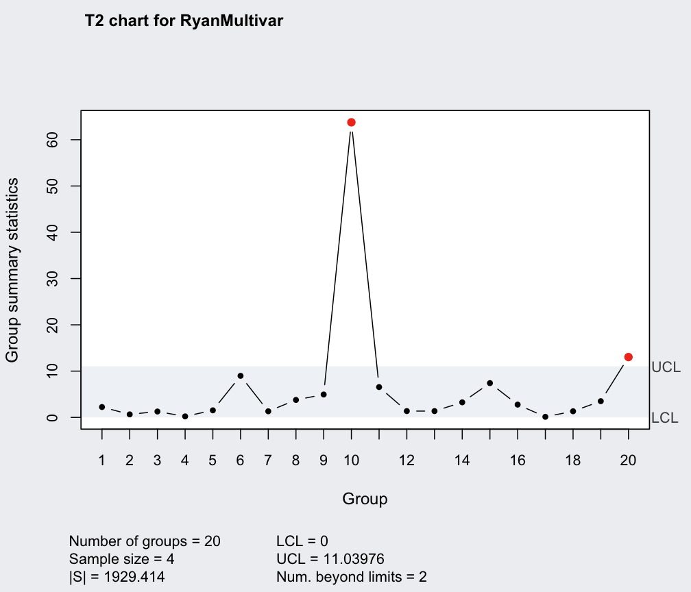 summary(q)
#> ── Multivariate Quality Control Chart ────────────
#>
#> Chart type = T2
#> Data (phase I) = RyanMultivar
#> Number of groups = 20
#> Group sample size = 4
#> Center =
#> X1 X2
#> 60.3750 18.4875
#> Covariance matrix =
#> X1 X2
#> X1 222.0333 103.11667
#> X2 103.1167 56.57917
#> |S| = 1929.414
#>
#> Control limits:
#> LCL UCL
#> 0 11.03976
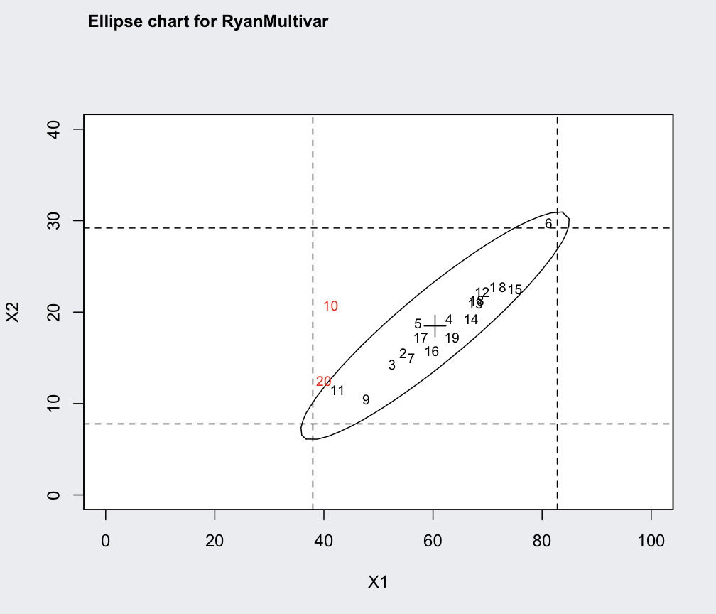
ellipseChart(q)
summary(q)
#> ── Multivariate Quality Control Chart ────────────
#>
#> Chart type = T2
#> Data (phase I) = RyanMultivar
#> Number of groups = 20
#> Group sample size = 4
#> Center =
#> X1 X2
#> 60.3750 18.4875
#> Covariance matrix =
#> X1 X2
#> X1 222.0333 103.11667
#> X2 103.1167 56.57917
#> |S| = 1929.414
#>
#> Control limits:
#> LCL UCL
#> 0 11.03976
ellipseChart(q)
 ellipseChart(q, show.id = TRUE)
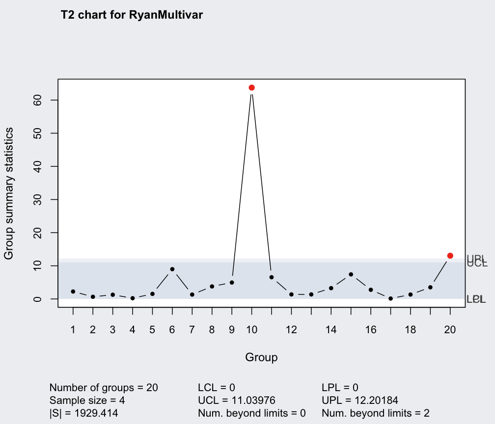
 q = mqcc(RyanMultivar, type = "T2", pred.limits = TRUE)
 # Xbar-charts for single variables computed adjusting the
# confidence level of the T^2 chart:
q1 = with(RyanMultivar,
qcc(X1, type = "xbar", confidence.level = q$confidence.level^(1/2)))
summary(q1)
#> ── Quality Control Chart ─────────────────────────
#>
#> Chart type = xbar
#> Data (phase I) = X1
#> Number of groups = 20
#> Group sample size = 4
#> Center of group statistics = 60.375
#> Standard deviation = 14.93443
#>
#> Control limits at nsigmas = 2.999977
#> LCL UCL
#> 37.97352 82.77648
q2 = with(RyanMultivar,
qcc(X2, type = "xbar", confidence.level = q$confidence.level^(1/2)))
summary(q2)
#> ── Quality Control Chart ─────────────────────────
#>
#> Chart type = xbar
#> Data (phase I) = X2
#> Number of groups = 20
#> Group sample size = 4
#> Center of group statistics = 18.4875
#> Standard deviation = 7.139388
#>
#> Control limits at nsigmas = 2.999977
#> LCL UCL
#> 7.7785 29.1965
require(MASS)
#> Loading required package: MASS
#>
#> Attaching package: ‘MASS’
#> The following object is masked from ‘package:patchwork’:
#>
#> area
# generate new "in control" data
Xnew = list(X1 = matrix(NA, 10, 4), X2 = matrix(NA, 10, 4))
for(i in 1:4)
{ x = mvrnorm(10, mu = q$center, Sigma = q$cov)
Xnew$X1[,i] = x[,1]
Xnew$X2[,i] = x[,2]
}
qq = mqcc(RyanMultivar, type = "T2", newdata = Xnew, pred.limits = TRUE)
# Xbar-charts for single variables computed adjusting the
# confidence level of the T^2 chart:
q1 = with(RyanMultivar,
qcc(X1, type = "xbar", confidence.level = q$confidence.level^(1/2)))
summary(q1)
#> ── Quality Control Chart ─────────────────────────
#>
#> Chart type = xbar
#> Data (phase I) = X1
#> Number of groups = 20
#> Group sample size = 4
#> Center of group statistics = 60.375
#> Standard deviation = 14.93443
#>
#> Control limits at nsigmas = 2.999977
#> LCL UCL
#> 37.97352 82.77648
q2 = with(RyanMultivar,
qcc(X2, type = "xbar", confidence.level = q$confidence.level^(1/2)))
summary(q2)
#> ── Quality Control Chart ─────────────────────────
#>
#> Chart type = xbar
#> Data (phase I) = X2
#> Number of groups = 20
#> Group sample size = 4
#> Center of group statistics = 18.4875
#> Standard deviation = 7.139388
#>
#> Control limits at nsigmas = 2.999977
#> LCL UCL
#> 7.7785 29.1965
require(MASS)
#> Loading required package: MASS
#>
#> Attaching package: ‘MASS’
#> The following object is masked from ‘package:patchwork’:
#>
#> area
# generate new "in control" data
Xnew = list(X1 = matrix(NA, 10, 4), X2 = matrix(NA, 10, 4))
for(i in 1:4)
{ x = mvrnorm(10, mu = q$center, Sigma = q$cov)
Xnew$X1[,i] = x[,1]
Xnew$X2[,i] = x[,2]
}
qq = mqcc(RyanMultivar, type = "T2", newdata = Xnew, pred.limits = TRUE)
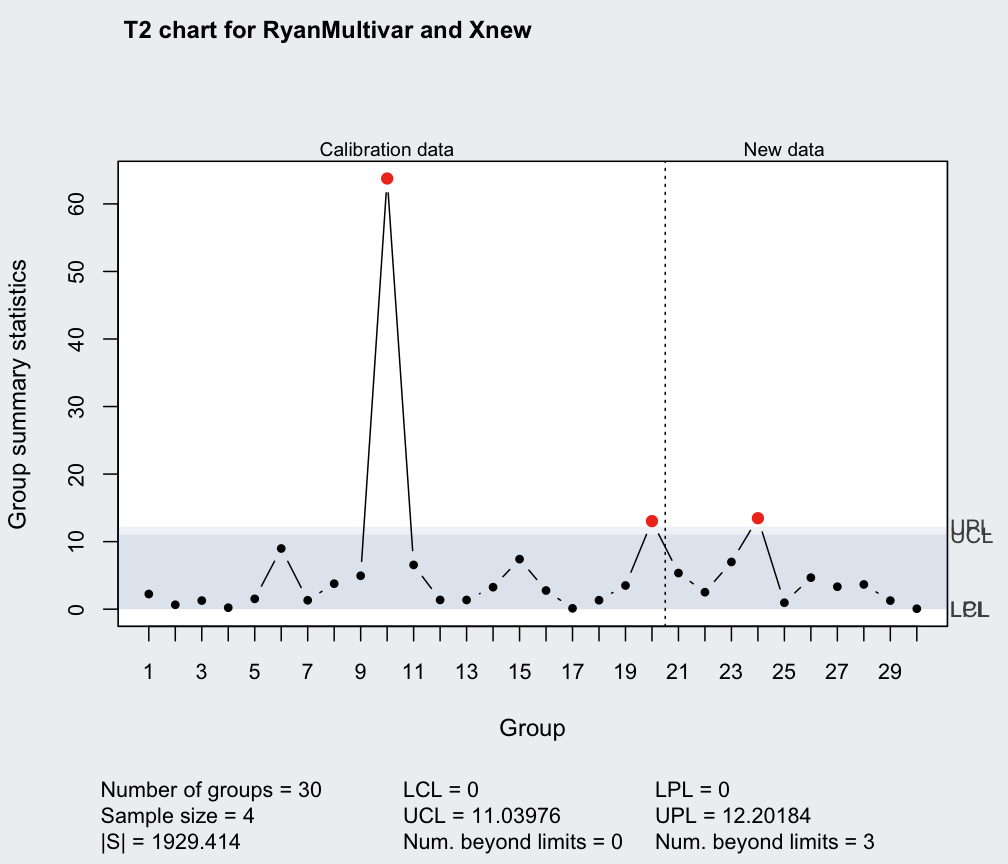
 summary(qq)
#> ── Multivariate Quality Control Chart ────────────
#>
#> Chart type = T2
#> Data (phase I) = RyanMultivar
#> Number of groups = 20
#> Group sample size = 4
#> Center =
#> X1 X2
#> 60.3750 18.4875
#> Covariance matrix =
#> X1 X2
#> X1 222.0333 103.11667
#> X2 103.1167 56.57917
#> |S| = 1929.414
#>
#> New data (phase II) = Xnew
#> Number of groups = 10
#> Group sample size = 4
#>
#> Control limits:
#> LCL UCL
#> 0 11.03976
#>
#> Prediction limits:
#> LPL UPL
#> 0 12.20184
# generate new "out of control" data
Xnew = list(X1 = matrix(NA, 10, 4), X2 = matrix(NA, 10, 4))
for(i in 1:4)
{ x = mvrnorm(10, mu = 1.2*q$center, Sigma = q$cov)
Xnew$X1[,i] = x[,1]
Xnew$X2[,i] = x[,2]
}
qq = mqcc(RyanMultivar, type = "T2", newdata = Xnew, pred.limits = TRUE)
summary(qq)
#> ── Multivariate Quality Control Chart ────────────
#>
#> Chart type = T2
#> Data (phase I) = RyanMultivar
#> Number of groups = 20
#> Group sample size = 4
#> Center =
#> X1 X2
#> 60.3750 18.4875
#> Covariance matrix =
#> X1 X2
#> X1 222.0333 103.11667
#> X2 103.1167 56.57917
#> |S| = 1929.414
#>
#> New data (phase II) = Xnew
#> Number of groups = 10
#> Group sample size = 4
#>
#> Control limits:
#> LCL UCL
#> 0 11.03976
#>
#> Prediction limits:
#> LPL UPL
#> 0 12.20184
# generate new "out of control" data
Xnew = list(X1 = matrix(NA, 10, 4), X2 = matrix(NA, 10, 4))
for(i in 1:4)
{ x = mvrnorm(10, mu = 1.2*q$center, Sigma = q$cov)
Xnew$X1[,i] = x[,1]
Xnew$X2[,i] = x[,2]
}
qq = mqcc(RyanMultivar, type = "T2", newdata = Xnew, pred.limits = TRUE)
 summary(qq)
#> ── Multivariate Quality Control Chart ────────────
#>
#> Chart type = T2
#> Data (phase I) = RyanMultivar
#> Number of groups = 20
#> Group sample size = 4
#> Center =
#> X1 X2
#> 60.3750 18.4875
#> Covariance matrix =
#> X1 X2
#> X1 222.0333 103.11667
#> X2 103.1167 56.57917
#> |S| = 1929.414
#>
#> New data (phase II) = Xnew
#> Number of groups = 10
#> Group sample size = 4
#>
#> Control limits:
#> LCL UCL
#> 0 11.03976
#>
#> Prediction limits:
#> LPL UPL
#> 0 12.20184
##
## Individual observations data
##
data(boiler)
str(boiler)
#> 'data.frame': 25 obs. of 8 variables:
#> $ t1: int 507 512 520 520 530 528 522 527 533 530 ...
#> $ t2: int 516 513 512 514 515 516 513 509 514 512 ...
#> $ t3: int 527 533 537 538 542 541 537 537 528 538 ...
#> $ t4: int 516 518 518 516 525 524 518 521 529 524 ...
#> $ t5: int 499 502 503 504 504 505 503 504 508 507 ...
#> $ t6: int 512 510 512 517 512 514 512 508 512 512 ...
#> $ t7: int 472 476 480 480 481 482 479 478 482 482 ...
#> $ t8: int 477 475 477 479 477 480 477 472 477 477 ...
q = mqcc(boiler, type = "T2.single", confidence.level = 0.999)
summary(qq)
#> ── Multivariate Quality Control Chart ────────────
#>
#> Chart type = T2
#> Data (phase I) = RyanMultivar
#> Number of groups = 20
#> Group sample size = 4
#> Center =
#> X1 X2
#> 60.3750 18.4875
#> Covariance matrix =
#> X1 X2
#> X1 222.0333 103.11667
#> X2 103.1167 56.57917
#> |S| = 1929.414
#>
#> New data (phase II) = Xnew
#> Number of groups = 10
#> Group sample size = 4
#>
#> Control limits:
#> LCL UCL
#> 0 11.03976
#>
#> Prediction limits:
#> LPL UPL
#> 0 12.20184
##
## Individual observations data
##
data(boiler)
str(boiler)
#> 'data.frame': 25 obs. of 8 variables:
#> $ t1: int 507 512 520 520 530 528 522 527 533 530 ...
#> $ t2: int 516 513 512 514 515 516 513 509 514 512 ...
#> $ t3: int 527 533 537 538 542 541 537 537 528 538 ...
#> $ t4: int 516 518 518 516 525 524 518 521 529 524 ...
#> $ t5: int 499 502 503 504 504 505 503 504 508 507 ...
#> $ t6: int 512 510 512 517 512 514 512 508 512 512 ...
#> $ t7: int 472 476 480 480 481 482 479 478 482 482 ...
#> $ t8: int 477 475 477 479 477 480 477 472 477 477 ...
q = mqcc(boiler, type = "T2.single", confidence.level = 0.999)
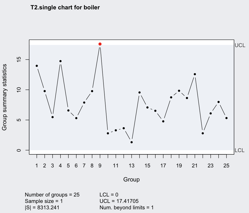 summary(q)
#> ── Multivariate Quality Control Chart ────────────
#>
#> Chart type = T2.single
#> Data (phase I) = boiler
#> Number of groups = 25
#> Group sample size = 1
#> Center =
#> t1 t2 t3 t4 t5 t6 t7 t8
#> 525.00 513.56 538.92 521.68 503.80 512.44 478.72 477.24
#> Covariance matrix =
#> t1 t2 t3 t4 t5 t6 t7
#> t1 54.0000000 0.9583333 20.583333 31.2916667 20.3333333 -2.2916667 20.3750000
#> t2 0.9583333 4.8400000 2.963333 2.6866667 0.3250000 3.0766667 0.7050000
#> t3 20.5833333 2.9633333 22.993333 10.0566667 4.9833333 2.0366667 6.4766667
#> t4 31.2916667 2.6866667 10.056667 22.3100000 13.5583333 -2.2700000 12.6983333
#> t5 20.3333333 0.3250000 4.983333 13.5583333 11.4166667 -1.6583333 10.6500000
#> t6 -2.2916667 3.0766667 2.036667 -2.2700000 -1.6583333 4.5066667 -0.7466667
#> t7 20.3750000 0.7050000 6.476667 12.6983333 10.6500000 -0.7466667 11.6266667
#> t8 0.2083333 3.4433333 2.770000 0.1633333 -0.2833333 3.7233333 0.5283333
#> t8
#> t1 0.2083333
#> t2 3.4433333
#> t3 2.7700000
#> t4 0.1633333
#> t5 -0.2833333
#> t6 3.7233333
#> t7 0.5283333
#> t8 3.8566667
#> |S| = 8313.241
#>
#> Control limits:
#> LCL UCL
#> 0 17.41705
# generate new "in control" data
boilerNew = mvrnorm(10, mu = q$center, Sigma = q$cov)
qq = mqcc(boiler, type = "T2.single", confidence.level = 0.999,
newdata = boilerNew, pred.limits = TRUE)
summary(q)
#> ── Multivariate Quality Control Chart ────────────
#>
#> Chart type = T2.single
#> Data (phase I) = boiler
#> Number of groups = 25
#> Group sample size = 1
#> Center =
#> t1 t2 t3 t4 t5 t6 t7 t8
#> 525.00 513.56 538.92 521.68 503.80 512.44 478.72 477.24
#> Covariance matrix =
#> t1 t2 t3 t4 t5 t6 t7
#> t1 54.0000000 0.9583333 20.583333 31.2916667 20.3333333 -2.2916667 20.3750000
#> t2 0.9583333 4.8400000 2.963333 2.6866667 0.3250000 3.0766667 0.7050000
#> t3 20.5833333 2.9633333 22.993333 10.0566667 4.9833333 2.0366667 6.4766667
#> t4 31.2916667 2.6866667 10.056667 22.3100000 13.5583333 -2.2700000 12.6983333
#> t5 20.3333333 0.3250000 4.983333 13.5583333 11.4166667 -1.6583333 10.6500000
#> t6 -2.2916667 3.0766667 2.036667 -2.2700000 -1.6583333 4.5066667 -0.7466667
#> t7 20.3750000 0.7050000 6.476667 12.6983333 10.6500000 -0.7466667 11.6266667
#> t8 0.2083333 3.4433333 2.770000 0.1633333 -0.2833333 3.7233333 0.5283333
#> t8
#> t1 0.2083333
#> t2 3.4433333
#> t3 2.7700000
#> t4 0.1633333
#> t5 -0.2833333
#> t6 3.7233333
#> t7 0.5283333
#> t8 3.8566667
#> |S| = 8313.241
#>
#> Control limits:
#> LCL UCL
#> 0 17.41705
# generate new "in control" data
boilerNew = mvrnorm(10, mu = q$center, Sigma = q$cov)
qq = mqcc(boiler, type = "T2.single", confidence.level = 0.999,
newdata = boilerNew, pred.limits = TRUE)
 summary(qq)
#> ── Multivariate Quality Control Chart ────────────
#>
#> Chart type = T2.single
#> Data (phase I) = boiler
#> Number of groups = 25
#> Group sample size = 1
#> Center =
#> t1 t2 t3 t4 t5 t6 t7 t8
#> 525.00 513.56 538.92 521.68 503.80 512.44 478.72 477.24
#> Covariance matrix =
#> t1 t2 t3 t4 t5 t6 t7
#> t1 54.0000000 0.9583333 20.583333 31.2916667 20.3333333 -2.2916667 20.3750000
#> t2 0.9583333 4.8400000 2.963333 2.6866667 0.3250000 3.0766667 0.7050000
#> t3 20.5833333 2.9633333 22.993333 10.0566667 4.9833333 2.0366667 6.4766667
#> t4 31.2916667 2.6866667 10.056667 22.3100000 13.5583333 -2.2700000 12.6983333
#> t5 20.3333333 0.3250000 4.983333 13.5583333 11.4166667 -1.6583333 10.6500000
#> t6 -2.2916667 3.0766667 2.036667 -2.2700000 -1.6583333 4.5066667 -0.7466667
#> t7 20.3750000 0.7050000 6.476667 12.6983333 10.6500000 -0.7466667 11.6266667
#> t8 0.2083333 3.4433333 2.770000 0.1633333 -0.2833333 3.7233333 0.5283333
#> t8
#> t1 0.2083333
#> t2 3.4433333
#> t3 2.7700000
#> t4 0.1633333
#> t5 -0.2833333
#> t6 3.7233333
#> t7 0.5283333
#> t8 3.8566667
#> |S| = 8313.241
#>
#> New data (phase II) = boilerNew
#> Number of groups = 10
#> Group sample size = 1
#>
#> Control limits:
#> LCL UCL
#> 0 17.41705
#>
#> Prediction limits:
#> LPL UPL
#> 0 70.02943
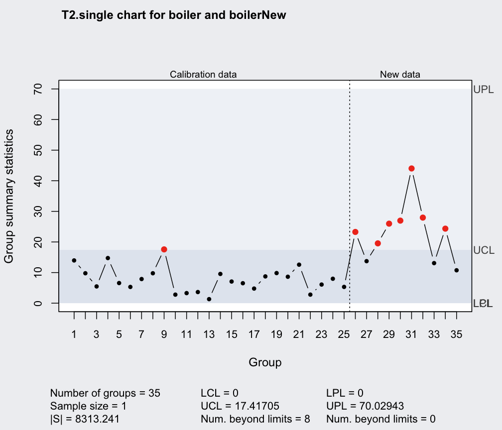
# generate new "out of control" data
boilerNew = mvrnorm(10, mu = 1.01*q$center, Sigma = q$cov)
qq = mqcc(boiler, type = "T2.single", confidence.level = 0.999,
newdata = boilerNew, pred.limits = TRUE)
summary(qq)
#> ── Multivariate Quality Control Chart ────────────
#>
#> Chart type = T2.single
#> Data (phase I) = boiler
#> Number of groups = 25
#> Group sample size = 1
#> Center =
#> t1 t2 t3 t4 t5 t6 t7 t8
#> 525.00 513.56 538.92 521.68 503.80 512.44 478.72 477.24
#> Covariance matrix =
#> t1 t2 t3 t4 t5 t6 t7
#> t1 54.0000000 0.9583333 20.583333 31.2916667 20.3333333 -2.2916667 20.3750000
#> t2 0.9583333 4.8400000 2.963333 2.6866667 0.3250000 3.0766667 0.7050000
#> t3 20.5833333 2.9633333 22.993333 10.0566667 4.9833333 2.0366667 6.4766667
#> t4 31.2916667 2.6866667 10.056667 22.3100000 13.5583333 -2.2700000 12.6983333
#> t5 20.3333333 0.3250000 4.983333 13.5583333 11.4166667 -1.6583333 10.6500000
#> t6 -2.2916667 3.0766667 2.036667 -2.2700000 -1.6583333 4.5066667 -0.7466667
#> t7 20.3750000 0.7050000 6.476667 12.6983333 10.6500000 -0.7466667 11.6266667
#> t8 0.2083333 3.4433333 2.770000 0.1633333 -0.2833333 3.7233333 0.5283333
#> t8
#> t1 0.2083333
#> t2 3.4433333
#> t3 2.7700000
#> t4 0.1633333
#> t5 -0.2833333
#> t6 3.7233333
#> t7 0.5283333
#> t8 3.8566667
#> |S| = 8313.241
#>
#> New data (phase II) = boilerNew
#> Number of groups = 10
#> Group sample size = 1
#>
#> Control limits:
#> LCL UCL
#> 0 17.41705
#>
#> Prediction limits:
#> LPL UPL
#> 0 70.02943
# generate new "out of control" data
boilerNew = mvrnorm(10, mu = 1.01*q$center, Sigma = q$cov)
qq = mqcc(boiler, type = "T2.single", confidence.level = 0.999,
newdata = boilerNew, pred.limits = TRUE)
 summary(qq)
#> ── Multivariate Quality Control Chart ────────────
#>
#> Chart type = T2.single
#> Data (phase I) = boiler
#> Number of groups = 25
#> Group sample size = 1
#> Center =
#> t1 t2 t3 t4 t5 t6 t7 t8
#> 525.00 513.56 538.92 521.68 503.80 512.44 478.72 477.24
#> Covariance matrix =
#> t1 t2 t3 t4 t5 t6 t7
#> t1 54.0000000 0.9583333 20.583333 31.2916667 20.3333333 -2.2916667 20.3750000
#> t2 0.9583333 4.8400000 2.963333 2.6866667 0.3250000 3.0766667 0.7050000
#> t3 20.5833333 2.9633333 22.993333 10.0566667 4.9833333 2.0366667 6.4766667
#> t4 31.2916667 2.6866667 10.056667 22.3100000 13.5583333 -2.2700000 12.6983333
#> t5 20.3333333 0.3250000 4.983333 13.5583333 11.4166667 -1.6583333 10.6500000
#> t6 -2.2916667 3.0766667 2.036667 -2.2700000 -1.6583333 4.5066667 -0.7466667
#> t7 20.3750000 0.7050000 6.476667 12.6983333 10.6500000 -0.7466667 11.6266667
#> t8 0.2083333 3.4433333 2.770000 0.1633333 -0.2833333 3.7233333 0.5283333
#> t8
#> t1 0.2083333
#> t2 3.4433333
#> t3 2.7700000
#> t4 0.1633333
#> t5 -0.2833333
#> t6 3.7233333
#> t7 0.5283333
#> t8 3.8566667
#> |S| = 8313.241
#>
#> New data (phase II) = boilerNew
#> Number of groups = 10
#> Group sample size = 1
#>
#> Control limits:
#> LCL UCL
#> 0 17.41705
#>
#> Prediction limits:
#> LPL UPL
#> 0 70.02943
# provides "robust" estimates of means and covariance matrix
rob = cov.rob(boiler)
qrob = mqcc(boiler, type = "T2.single", center = rob$center, cov = rob$cov)
summary(qq)
#> ── Multivariate Quality Control Chart ────────────
#>
#> Chart type = T2.single
#> Data (phase I) = boiler
#> Number of groups = 25
#> Group sample size = 1
#> Center =
#> t1 t2 t3 t4 t5 t6 t7 t8
#> 525.00 513.56 538.92 521.68 503.80 512.44 478.72 477.24
#> Covariance matrix =
#> t1 t2 t3 t4 t5 t6 t7
#> t1 54.0000000 0.9583333 20.583333 31.2916667 20.3333333 -2.2916667 20.3750000
#> t2 0.9583333 4.8400000 2.963333 2.6866667 0.3250000 3.0766667 0.7050000
#> t3 20.5833333 2.9633333 22.993333 10.0566667 4.9833333 2.0366667 6.4766667
#> t4 31.2916667 2.6866667 10.056667 22.3100000 13.5583333 -2.2700000 12.6983333
#> t5 20.3333333 0.3250000 4.983333 13.5583333 11.4166667 -1.6583333 10.6500000
#> t6 -2.2916667 3.0766667 2.036667 -2.2700000 -1.6583333 4.5066667 -0.7466667
#> t7 20.3750000 0.7050000 6.476667 12.6983333 10.6500000 -0.7466667 11.6266667
#> t8 0.2083333 3.4433333 2.770000 0.1633333 -0.2833333 3.7233333 0.5283333
#> t8
#> t1 0.2083333
#> t2 3.4433333
#> t3 2.7700000
#> t4 0.1633333
#> t5 -0.2833333
#> t6 3.7233333
#> t7 0.5283333
#> t8 3.8566667
#> |S| = 8313.241
#>
#> New data (phase II) = boilerNew
#> Number of groups = 10
#> Group sample size = 1
#>
#> Control limits:
#> LCL UCL
#> 0 17.41705
#>
#> Prediction limits:
#> LPL UPL
#> 0 70.02943
# provides "robust" estimates of means and covariance matrix
rob = cov.rob(boiler)
qrob = mqcc(boiler, type = "T2.single", center = rob$center, cov = rob$cov)
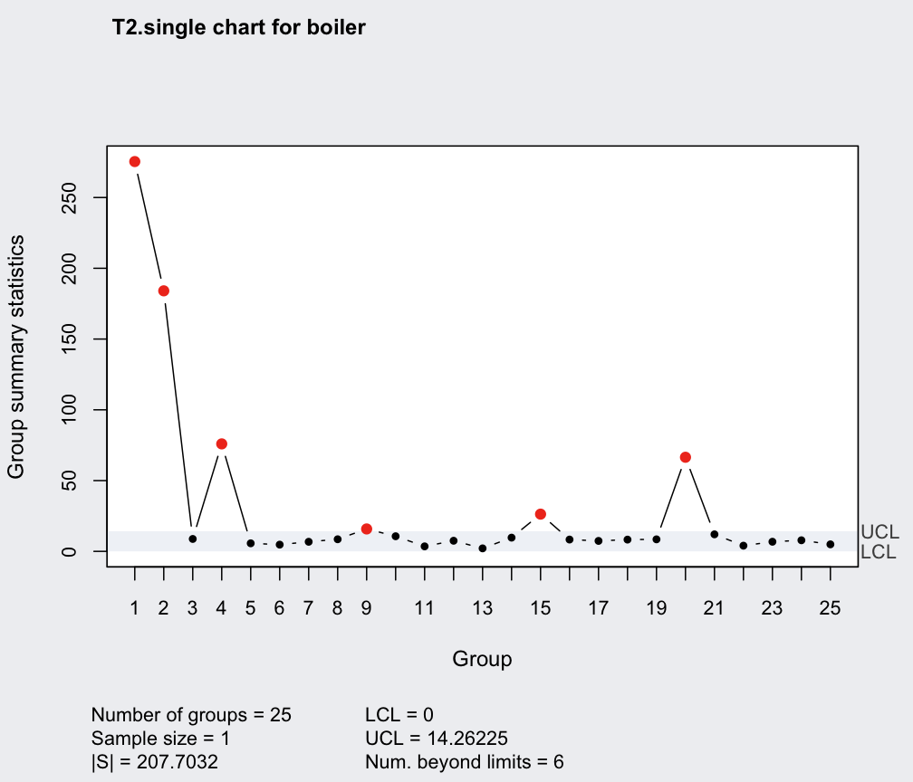 summary(qrob)
#> ── Multivariate Quality Control Chart ────────────
#>
#> Chart type = T2.single
#> Data (phase I) = boiler
#> Number of groups = 25
#> Group sample size = 1
#> Center =
#> t1 t2 t3 t4 t5 t6 t7 t8
#> 526.55 513.40 540.35 522.25 504.25 512.30 479.15 477.25
#> Covariance matrix =
#> t1 t2 t3 t4 t5 t6 t7
#> t1 34.5763158 3.400000 12.850000 25.5394737 16.3815789 -3.121053 15.1763158
#> t2 3.4000000 5.726316 5.589474 4.1578947 1.1052632 3.715789 1.7263158
#> t3 12.8500000 5.589474 11.186842 11.2763158 4.8552632 1.626316 4.6289474
#> t4 25.5394737 4.157895 11.276316 20.1973684 12.1973684 -1.552632 11.6447368
#> t5 16.3815789 1.105263 4.855263 12.1973684 9.4605263 -1.763158 9.2236842
#> t6 -3.1210526 3.715789 1.626316 -1.5526316 -1.7631579 4.115789 -1.3105263
#> t7 15.1763158 1.726316 4.628947 11.6447368 9.2236842 -1.310526 10.3447368
#> t8 -0.8289474 4.263158 2.539474 0.4605263 -0.3289474 3.921053 0.3289474
#> t8
#> t1 -0.8289474
#> t2 4.2631579
#> t3 2.5394737
#> t4 0.4605263
#> t5 -0.3289474
#> t6 3.9210526
#> t7 0.3289474
#> t8 4.4078947
#> |S| = 90.46966
#>
#> Control limits:
#> LCL UCL
#> 0 14.26225
summary(qrob)
#> ── Multivariate Quality Control Chart ────────────
#>
#> Chart type = T2.single
#> Data (phase I) = boiler
#> Number of groups = 25
#> Group sample size = 1
#> Center =
#> t1 t2 t3 t4 t5 t6 t7 t8
#> 526.55 513.40 540.35 522.25 504.25 512.30 479.15 477.25
#> Covariance matrix =
#> t1 t2 t3 t4 t5 t6 t7
#> t1 34.5763158 3.400000 12.850000 25.5394737 16.3815789 -3.121053 15.1763158
#> t2 3.4000000 5.726316 5.589474 4.1578947 1.1052632 3.715789 1.7263158
#> t3 12.8500000 5.589474 11.186842 11.2763158 4.8552632 1.626316 4.6289474
#> t4 25.5394737 4.157895 11.276316 20.1973684 12.1973684 -1.552632 11.6447368
#> t5 16.3815789 1.105263 4.855263 12.1973684 9.4605263 -1.763158 9.2236842
#> t6 -3.1210526 3.715789 1.626316 -1.5526316 -1.7631579 4.115789 -1.3105263
#> t7 15.1763158 1.726316 4.628947 11.6447368 9.2236842 -1.310526 10.3447368
#> t8 -0.8289474 4.263158 2.539474 0.4605263 -0.3289474 3.921053 0.3289474
#> t8
#> t1 -0.8289474
#> t2 4.2631579
#> t3 2.5394737
#> t4 0.4605263
#> t5 -0.3289474
#> t6 3.9210526
#> t7 0.3289474
#> t8 4.4078947
#> |S| = 90.46966
#>
#> Control limits:
#> LCL UCL
#> 0 14.26225