Quality Control Charts
qcc.RdCreate an object of class 'qcc' to perform statistical quality control. This object may then be used to plot Shewhart charts, drawing OC curves, computes capability indices, and more.
Usage
qcc(data,
    type = c("xbar", "R", "S", "xbar.one", "p", "np", "c", "u", "g"),
    sizes, center, std.dev, limits,
    newdata, newsizes,
    nsigmas = 3, confidence.level,
    rules = c(1,4), ...)

# S3 method for class 'qcc'
print(x, digits = getOption("digits"), ...)

# S3 method for class 'qcc'
plot(x,
     xtime = NULL,
     add.stats = qcc.options("add.stats"),
     chart.all = qcc.options("chart.all"),
     fill = qcc.options("fill"),
     label.center = "CL",
     label.limits = c("LCL ", "UCL"),
     title, xlab, ylab, xlim, ylim,
     digits = getOption("digits"), ...)
Arguments
- data
a data frame, a matrix or a vector containing observed data for the variable to chart. Each row of a data frame or a matrix, and each value of a vector, refers to a sample or ”rationale group”.
- type
a character string specifying the group statistics to compute.
Available methods are:Statistic charted Chart description "xbar"mean means of a continuous process variable "R"range ranges of a continuous process variable "S"standard deviation standard deviations of a continuous variable "xbar.one"mean one-at-time data of a continuous process variable "p"proportion proportion of nonconforming units "np"count number of nonconforming units "c"count nonconformities per unit "u"count average nonconformities per unit "g"count number of non-events between events Furthermore, a user specified type of chart, say
"newchart", can be provided. This requires the definition of"stats.newchart","sd.newchart", and"limits.newchart". As an example, seestats.xbar.- sizes
a value or a vector of values specifying the sample sizes associated with each group. For continuous data provided as data frame or matrix the sample sizes are obtained counting the non-
NAelements of each row. For"p","np"and"u"charts the argumentsizesis required.- center
a value specifying the center of group statistics or the ”target” value of the process.
- std.dev
a value or an available method specifying the within-group standard deviation(s) of the process.
Several methods are available for estimating the standard deviation in case of a continuous process variable; seesd.xbar,sd.xbar.one,sd.R,sd.S.- limits
a two-values vector specifying control limits.
- newdata
a data frame, matrix or vector, as for the
dataargument, providing further data to plot but not included in the computations.- newsizes
a vector as for the
sizesargument providing further data sizes to plot but not included in the computations.- nsigmas
a numeric value specifying the number of sigmas to use for computing control limits. It is ignored when the
confidence.levelargument is provided.- confidence.level
a numeric value between 0 and 1 specifying the confidence level of the computed probability limits.
- rules
a value or a vector of values specifying the rules to apply to the chart. See
qccRulesfor possible values and their meaning.- xtime
a vector of date-time values as returned by
Sys.timeandSys.Date. If provided it is used for x-axis so it must be of the same length as the statistic charted.- add.stats
a logical value indicating whether statistics and other information should be printed at the bottom of the chart.
- chart.all
a logical value indicating whether both statistics for
dataand fornewdata(if given) should be plotted.- fill
a logical value specifying if the in-control area should be filled with the color specified in
qcc.options("zones")$fill.- label.center
a character specifying the label for center line.
- label.limits
a character vector specifying the labels for control limits.
- title
a character string specifying the main title. Set
title = NULLto remove the title.- xlab, ylab
a string giving the label for the x-axis and the y-axis.
- xlim, ylim
a numeric vector specifying the limits for the x-axis and the y-axis.
- digits
the number of significant digits to use.
- x
an object of class
'qcc'.- ...
additional arguments to be passed to the generic function.
References
Mason, R.L. and Young, J.C. (2002) Multivariate Statistical Process Control with Industrial Applications, SIAM.
Montgomery, D.C. (2013) Introduction to Statistical Quality Control, 7th ed. New York: John Wiley & Sons.
Ryan, T. P. (2011), Statistical Methods for Quality Improvement, 3rd ed. New York: John Wiley & Sons, Inc.
Scrucca, L. (2004). qcc: an R package for quality control charting and statistical process control. R News 4/1, 11-17.
Wetherill, G.B. and Brown, D.W. (1991) Statistical Process Control. New York: Chapman & Hall.
Examples
##
## Continuous data
##
data(pistonrings)
diameter = qccGroups(data = pistonrings, diameter, sample)
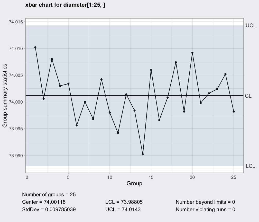
(q = qcc(diameter[1:25,], type="xbar"))
#> ── Quality Control Chart ─────────────────────────
#>
#> Chart type = xbar
#> Data (phase I) = diameter[1:25, ]
#> Number of groups = 25
#> Group sample size = 5
#> Center of group statistics = 74.00118
#> Standard deviation = 0.009785039
#>
#> Control limits at nsigmas = 3
#> LCL UCL
#> 73.98805 74.0143
plot(q)
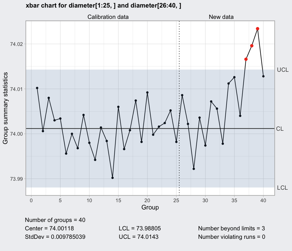
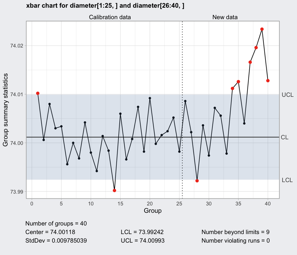
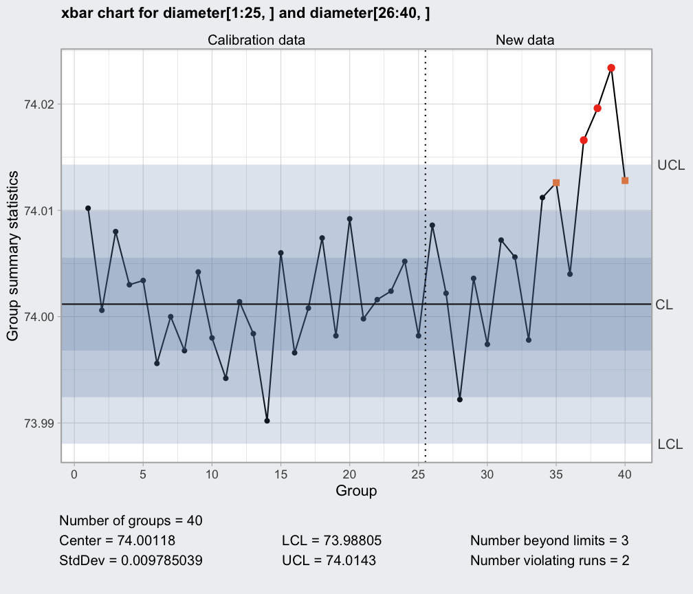
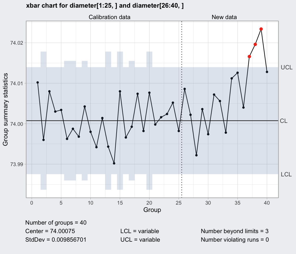
 (q = qcc(diameter[1:25,], type="xbar", newdata=diameter[26:40,]))
#> ── Quality Control Chart ─────────────────────────
#>
#> Chart type = xbar
#> Data (phase I) = diameter[1:25, ]
#> Number of groups = 25
#> Group sample size = 5
#> Center of group statistics = 74.00118
#> Standard deviation = 0.009785039
#>
#> New data (phase II) = diameter[26:40, ]
#> Number of groups = 15
#> Group sample size = 5
#>
#> Control limits at nsigmas = 3
#> LCL UCL
#> 73.98805 74.0143
plot(q)
(q = qcc(diameter[1:25,], type="xbar", newdata=diameter[26:40,]))
#> ── Quality Control Chart ─────────────────────────
#>
#> Chart type = xbar
#> Data (phase I) = diameter[1:25, ]
#> Number of groups = 25
#> Group sample size = 5
#> Center of group statistics = 74.00118
#> Standard deviation = 0.009785039
#>
#> New data (phase II) = diameter[26:40, ]
#> Number of groups = 15
#> Group sample size = 5
#>
#> Control limits at nsigmas = 3
#> LCL UCL
#> 73.98805 74.0143
plot(q)
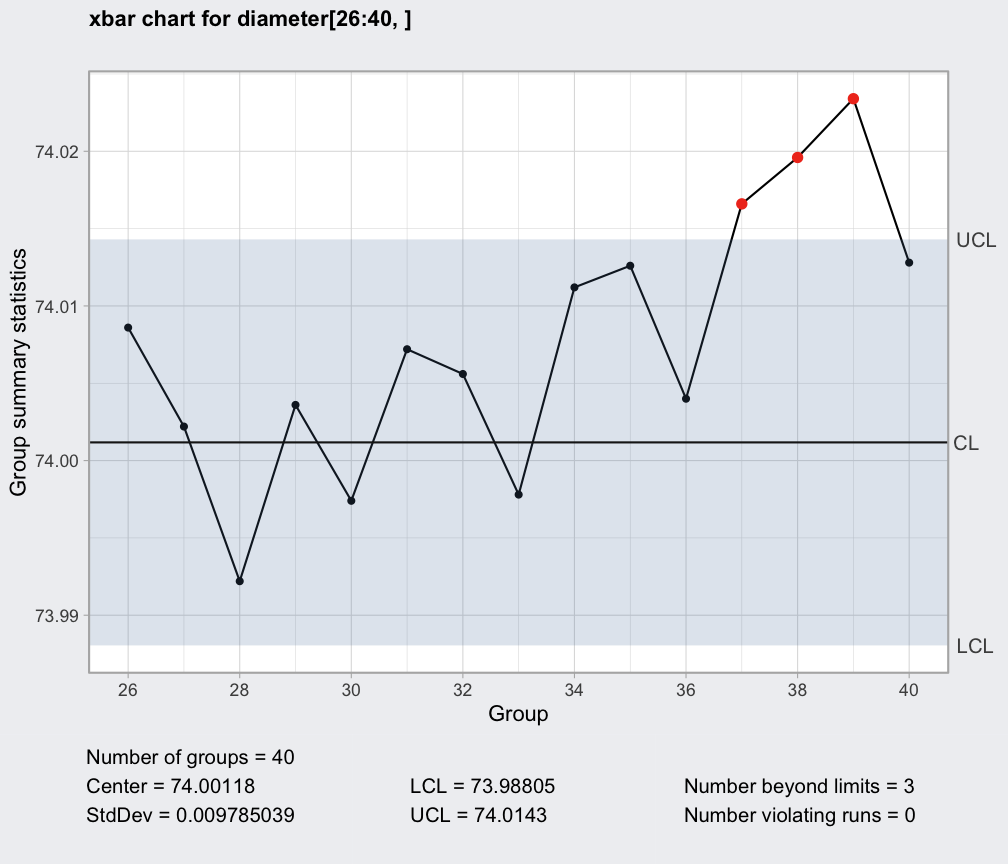
 q = qcc(diameter[1:25,], type="xbar", newdata=diameter[26:40,])
plot(q, chart.all=FALSE)
q = qcc(diameter[1:25,], type="xbar", newdata=diameter[26:40,])
plot(q, chart.all=FALSE)
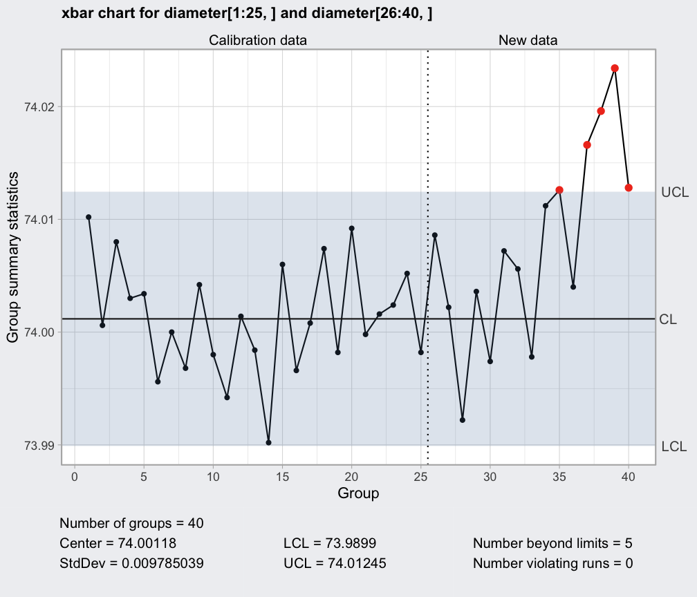
 plot(qcc(diameter[1:25,], type="xbar", newdata=diameter[26:40,], nsigmas=2))
 plot(qcc(diameter[1:25,], type="xbar", newdata=diameter[26:40,], confidence.level=0.99))
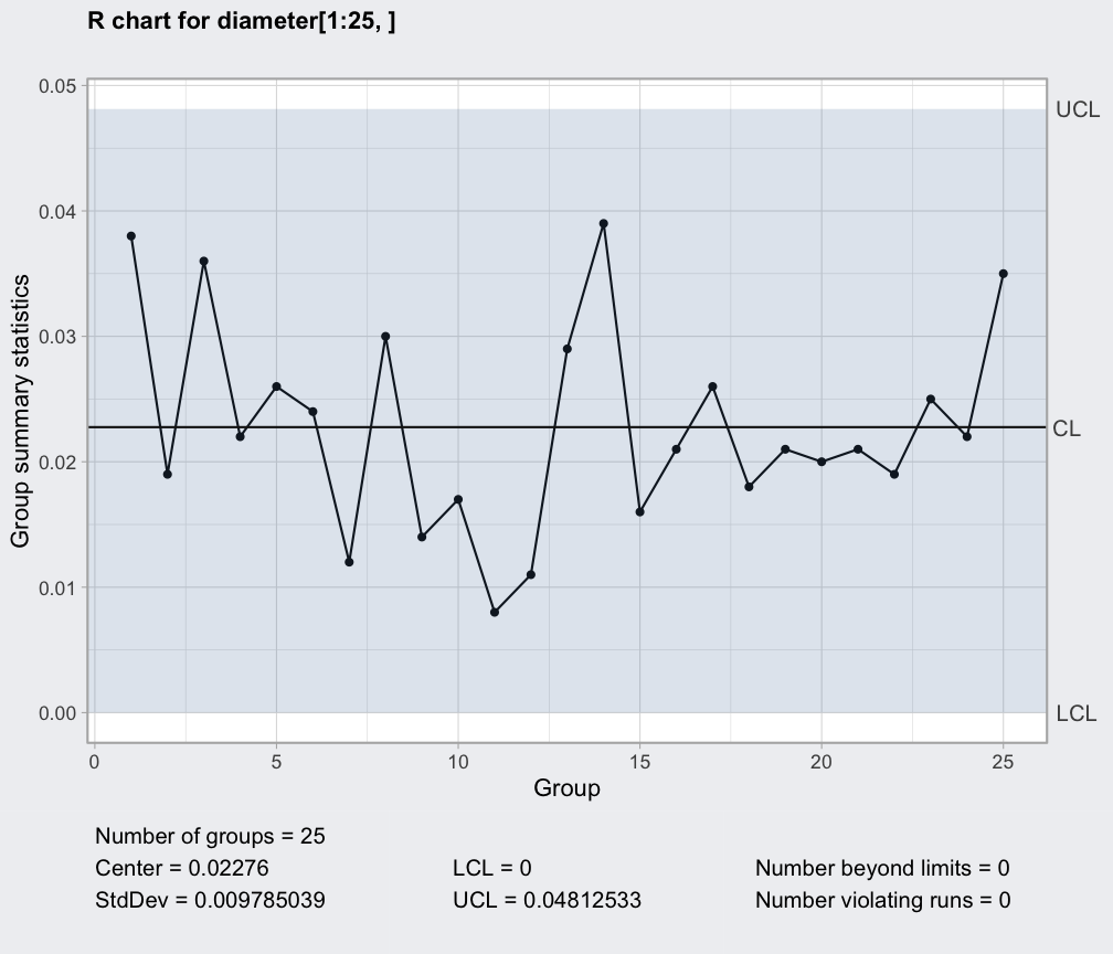
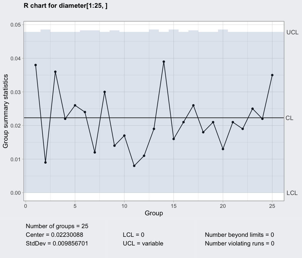
 q = qcc(diameter[1:25,], type="R")
q
#> ── Quality Control Chart ─────────────────────────
#>
#> Chart type = R
#> Data (phase I) = diameter[1:25, ]
#> Number of groups = 25
#> Group sample size = 5
#> Center of group statistics = 0.02276
#> Standard deviation = 0.009785039
#>
#> Control limits at nsigmas = 3
#> LCL UCL
#> 0 0.04812533
plot(q)
q = qcc(diameter[1:25,], type="R")
q
#> ── Quality Control Chart ─────────────────────────
#>
#> Chart type = R
#> Data (phase I) = diameter[1:25, ]
#> Number of groups = 25
#> Group sample size = 5
#> Center of group statistics = 0.02276
#> Standard deviation = 0.009785039
#>
#> Control limits at nsigmas = 3
#> LCL UCL
#> 0 0.04812533
plot(q)
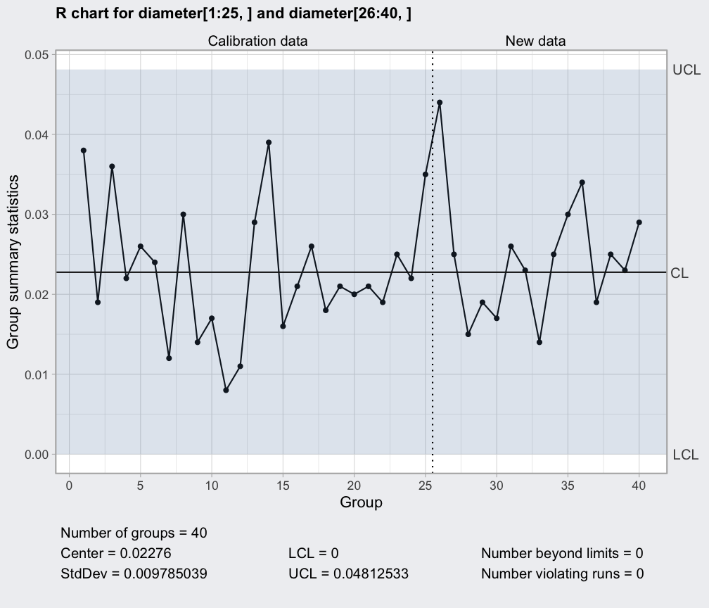
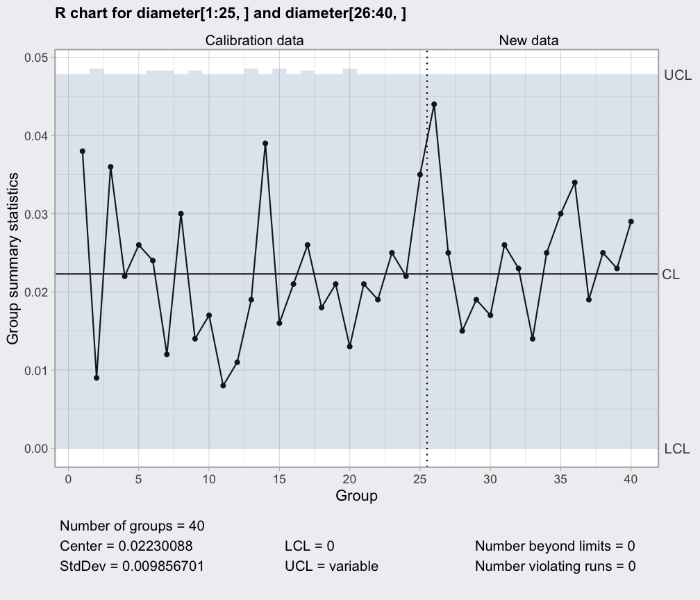
 plot(qcc(diameter[1:25,], type="R", newdata=diameter[26:40,]))
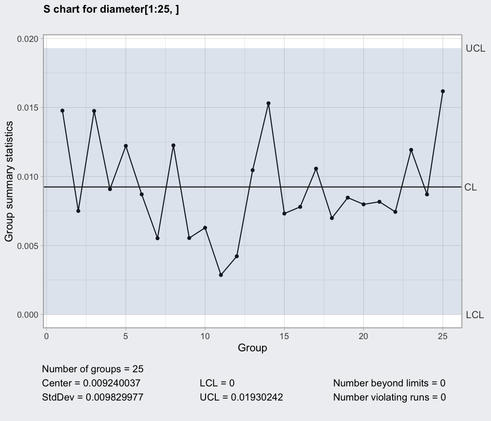
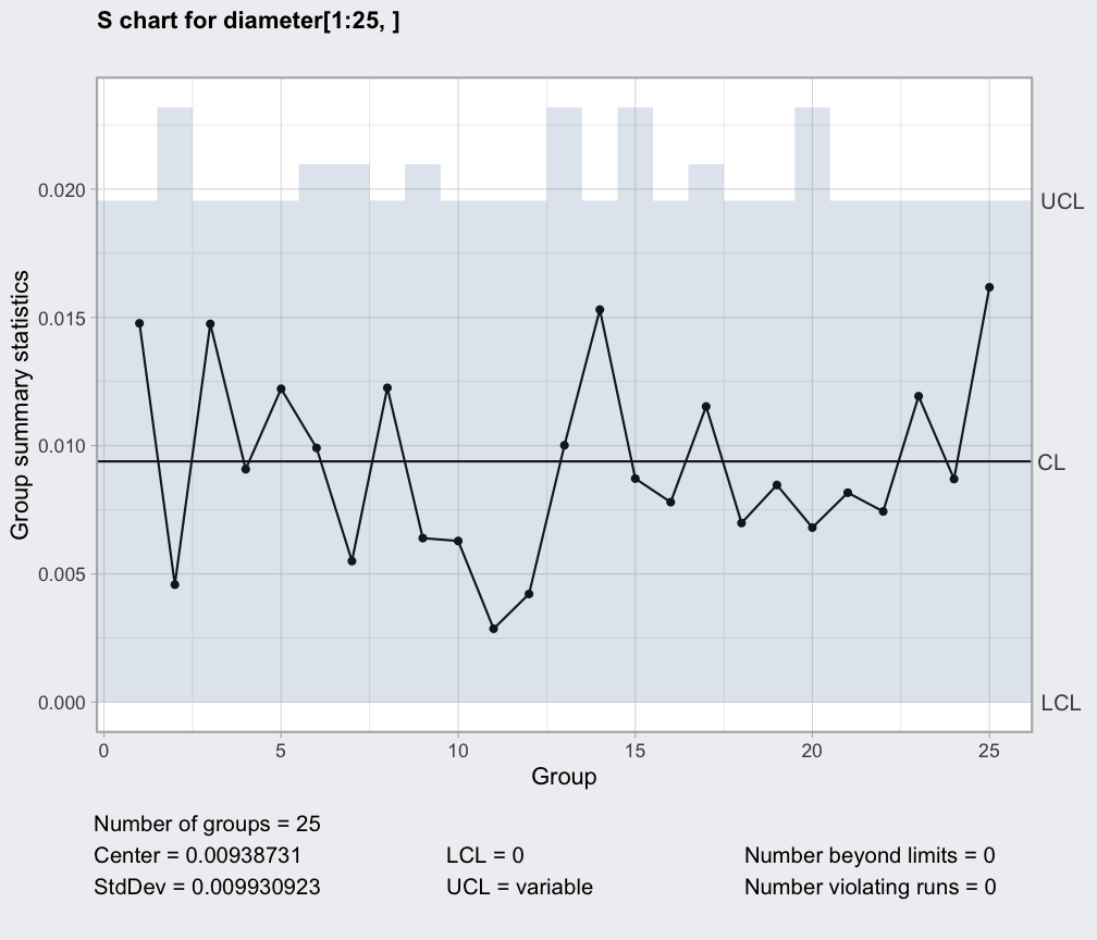
 plot(qcc(diameter[1:25,], type="S"))
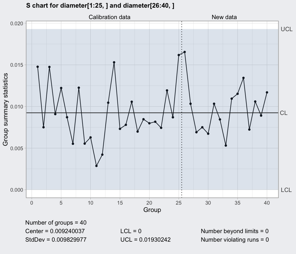
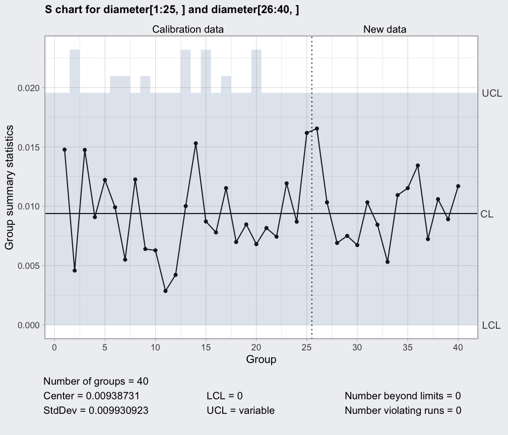
 plot(qcc(diameter[1:25,], type="S", newdata=diameter[26:40,]))
 plot(qcc(diameter[1:25,], type="xbar", newdata=diameter[26:40,], rules = 1:4))
 # variable control limits
out = c(9, 10, 30, 35, 45, 64, 65, 74, 75, 85, 99, 100)
diameter = qccGroups(data = pistonrings[-out,], diameter, sample)
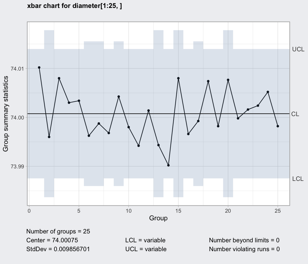
plot(qcc(diameter[1:25,], type="xbar"))
# variable control limits
out = c(9, 10, 30, 35, 45, 64, 65, 74, 75, 85, 99, 100)
diameter = qccGroups(data = pistonrings[-out,], diameter, sample)
plot(qcc(diameter[1:25,], type="xbar"))
 plot(qcc(diameter[1:25,], type="R"))
 plot(qcc(diameter[1:25,], type="S"))
 plot(qcc(diameter[1:25,], type="xbar", newdata=diameter[26:40,]))
 plot(qcc(diameter[1:25,], type="R", newdata=diameter[26:40,]))
 plot(qcc(diameter[1:25,], type="S", newdata=diameter[26:40,]))
 # to customize a Shewhart chart use
q = qcc(diameter[1:25, ], type = "xbar")
plot = plot(q, ylim = c(73.9, 74.1))
# returned object is of class "patchwork", then add geom_* layer to the first element
plot[[1]] <- plot[[1]] +
geom_hline(yintercept = c(73.95, 74.05), lty = 2)
plot
# to customize a Shewhart chart use
q = qcc(diameter[1:25, ], type = "xbar")
plot = plot(q, ylim = c(73.9, 74.1))
# returned object is of class "patchwork", then add geom_* layer to the first element
plot[[1]] <- plot[[1]] +
geom_hline(yintercept = c(73.95, 74.05), lty = 2)
plot
 ##
## Attribute data
##
data(orangejuice)
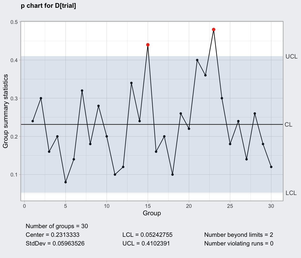
q = with(orangejuice,
qcc(D[trial], sizes=size[trial], type="p"))
q
#> ── Quality Control Chart ─────────────────────────
#>
#> Chart type = p
#> Data (phase I) = D[trial]
#> Number of groups = 30
#> Group sample size = 50
#> Center of group statistics = 0.2313333
#> Standard deviation = 0.05963526
#>
#> Control limits at nsigmas = 3
#> LCL UCL
#> 0.05242755 0.4102391
#> 0.05242755 0.4102391
#> :
#> 0.05242755 0.4102391
plot(q)
##
## Attribute data
##
data(orangejuice)
q = with(orangejuice,
qcc(D[trial], sizes=size[trial], type="p"))
q
#> ── Quality Control Chart ─────────────────────────
#>
#> Chart type = p
#> Data (phase I) = D[trial]
#> Number of groups = 30
#> Group sample size = 50
#> Center of group statistics = 0.2313333
#> Standard deviation = 0.05963526
#>
#> Control limits at nsigmas = 3
#> LCL UCL
#> 0.05242755 0.4102391
#> 0.05242755 0.4102391
#> :
#> 0.05242755 0.4102391
plot(q)
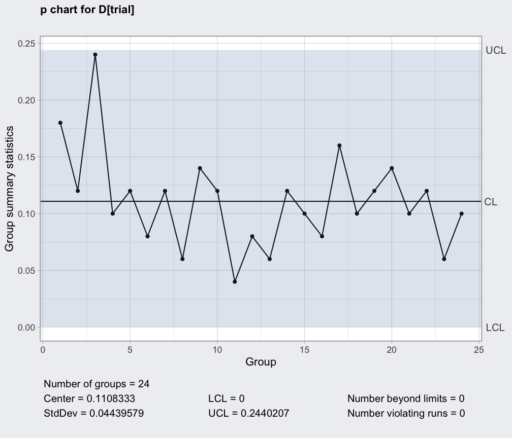
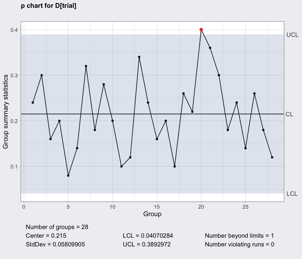 # remove out-of-control points (see help(orangejuice) for the reasons)
outofctrl = c(15,23)
q1 = with(orangejuice[-outofctrl,],
qcc(D[trial], sizes=size[trial], type="p"))
plot(q1)
# remove out-of-control points (see help(orangejuice) for the reasons)
outofctrl = c(15,23)
q1 = with(orangejuice[-outofctrl,],
qcc(D[trial], sizes=size[trial], type="p"))
plot(q1)
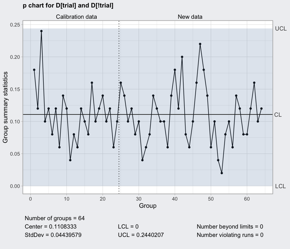
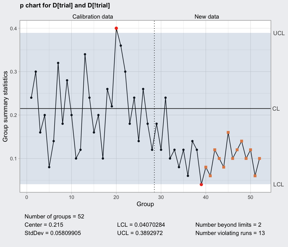 q1 = with(orangejuice[-outofctrl,],
qcc(D[trial], sizes=size[trial], type="p",
newdata=D[!trial], newsizes=size[!trial]))
plot(q1)
q1 = with(orangejuice[-outofctrl,],
qcc(D[trial], sizes=size[trial], type="p",
newdata=D[!trial], newsizes=size[!trial]))
plot(q1)
 data(orangejuice2)
q2 = with(orangejuice2,
qcc(D[trial], sizes=size[trial], type="p"))
plot(q2)
data(orangejuice2)
q2 = with(orangejuice2,
qcc(D[trial], sizes=size[trial], type="p"))
plot(q2)
 q2 = with(orangejuice2,
qcc(D[trial], sizes=size[trial], type="p",
newdata=D[!trial], newsizes=size[!trial]))
plot(q2)
q2 = with(orangejuice2,
qcc(D[trial], sizes=size[trial], type="p",
newdata=D[!trial], newsizes=size[!trial]))
plot(q2)
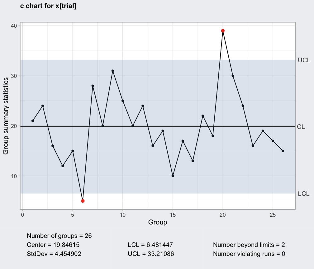 data(circuit)
plot(with(circuit, qcc(x[trial], sizes=size[trial], type="c")))
data(circuit)
plot(with(circuit, qcc(x[trial], sizes=size[trial], type="c")))
 # remove out-of-control points (see help(circuit) for the reasons)
outofctrl = c(15,23)
q1 = with(orangejuice[-outofctrl,],
qcc(D[trial], sizes=size[trial], type="p"))
plot(q1)
# remove out-of-control points (see help(circuit) for the reasons)
outofctrl = c(15,23)
q1 = with(orangejuice[-outofctrl,],
qcc(D[trial], sizes=size[trial], type="p"))
plot(q1)
 q1 = with(orangejuice[-outofctrl,],
qcc(D[trial], sizes=size[trial], type="p",
newdata=D[!trial], newsizes=size[!trial]))
plot(q1)
q1 = with(orangejuice[-outofctrl,],
qcc(D[trial], sizes=size[trial], type="p",
newdata=D[!trial], newsizes=size[!trial]))
plot(q1)
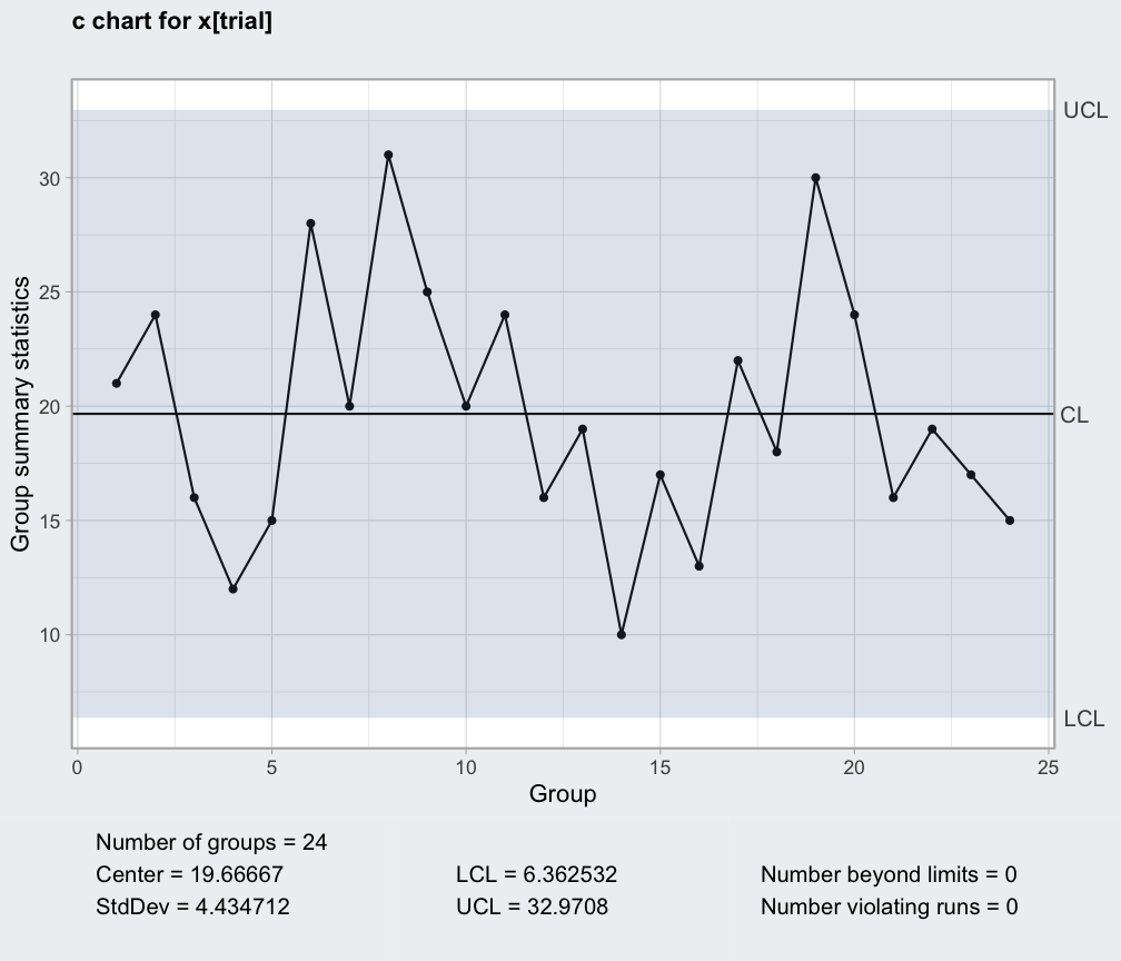 outofctrl = c(6,20)
q1 = with(circuit[-outofctrl,],
qcc(x[trial], sizes=size[trial], type="c"))
plot(q1)
outofctrl = c(6,20)
q1 = with(circuit[-outofctrl,],
qcc(x[trial], sizes=size[trial], type="c"))
plot(q1)
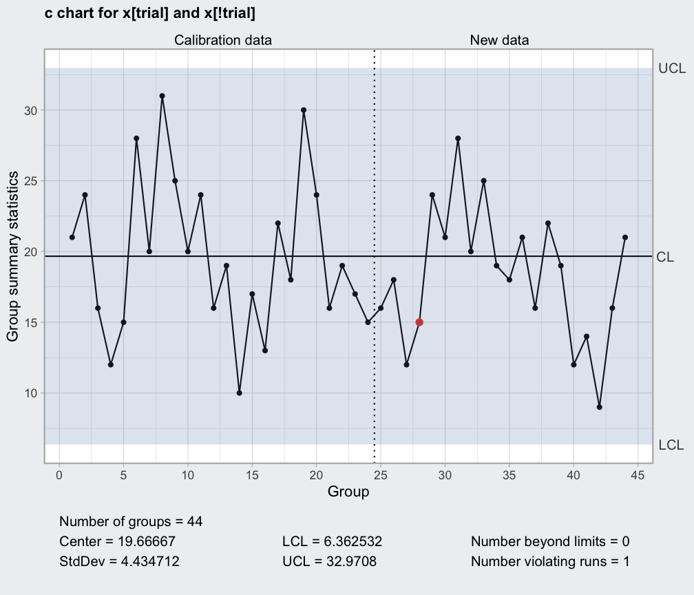 q1 = with(circuit[-outofctrl,],
qcc(x[trial], sizes=size[trial], type="c",
newdata = x[!trial], newsizes = size[!trial]))
plot(q1)
q1 = with(circuit[-outofctrl,],
qcc(x[trial], sizes=size[trial], type="c",
newdata = x[!trial], newsizes = size[!trial]))
plot(q1)
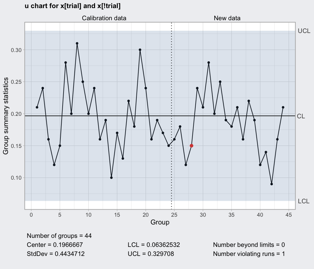 q1 = with(circuit[-outofctrl,],
qcc(x[trial], sizes=size[trial], type="u",
newdata = x[!trial], newsizes = size[!trial]))
plot(q1)
q1 = with(circuit[-outofctrl,],
qcc(x[trial], sizes=size[trial], type="u",
newdata = x[!trial], newsizes = size[!trial]))
plot(q1)
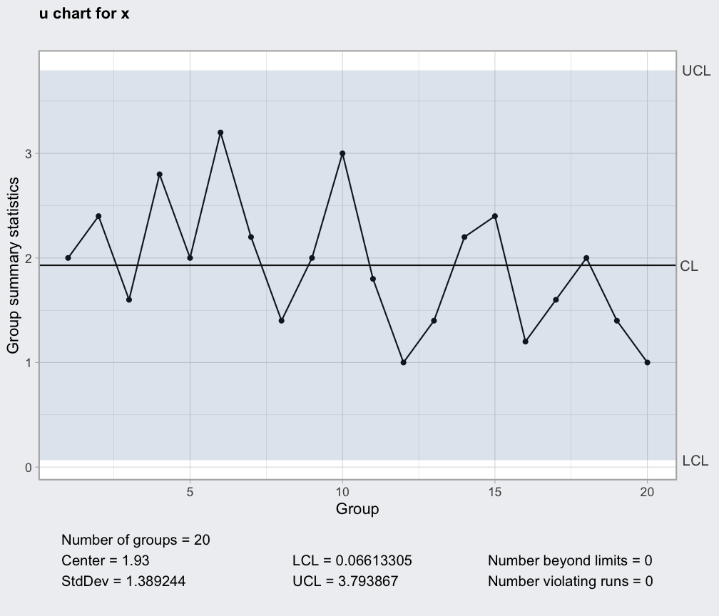 data(pcmanufact)
q1 = with(pcmanufact, qcc(x, sizes=size, type="u"))
q1
#> ── Quality Control Chart ─────────────────────────
#>
#> Chart type = u
#> Data (phase I) = x
#> Number of groups = 20
#> Group sample size = 5
#> Center of group statistics = 1.93
#> Standard deviation = 1.389244
#>
#> Control limits at nsigmas = 3
#> LCL UCL
#> 0.06613305 3.793867
plot(q1)
data(pcmanufact)
q1 = with(pcmanufact, qcc(x, sizes=size, type="u"))
q1
#> ── Quality Control Chart ─────────────────────────
#>
#> Chart type = u
#> Data (phase I) = x
#> Number of groups = 20
#> Group sample size = 5
#> Center of group statistics = 1.93
#> Standard deviation = 1.389244
#>
#> Control limits at nsigmas = 3
#> LCL UCL
#> 0.06613305 3.793867
plot(q1)
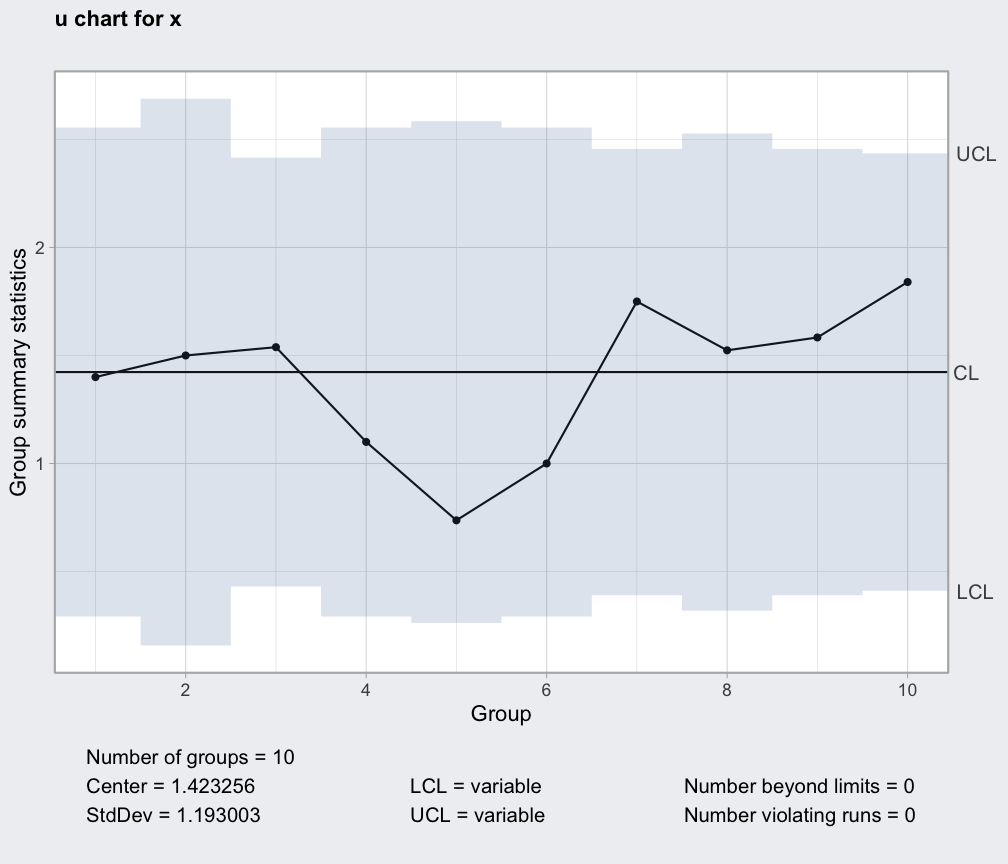 data(dyedcloth)
# variable control limits
plot(with(dyedcloth, qcc(x, sizes=size, type="u")))
data(dyedcloth)
# variable control limits
plot(with(dyedcloth, qcc(x, sizes=size, type="u")))
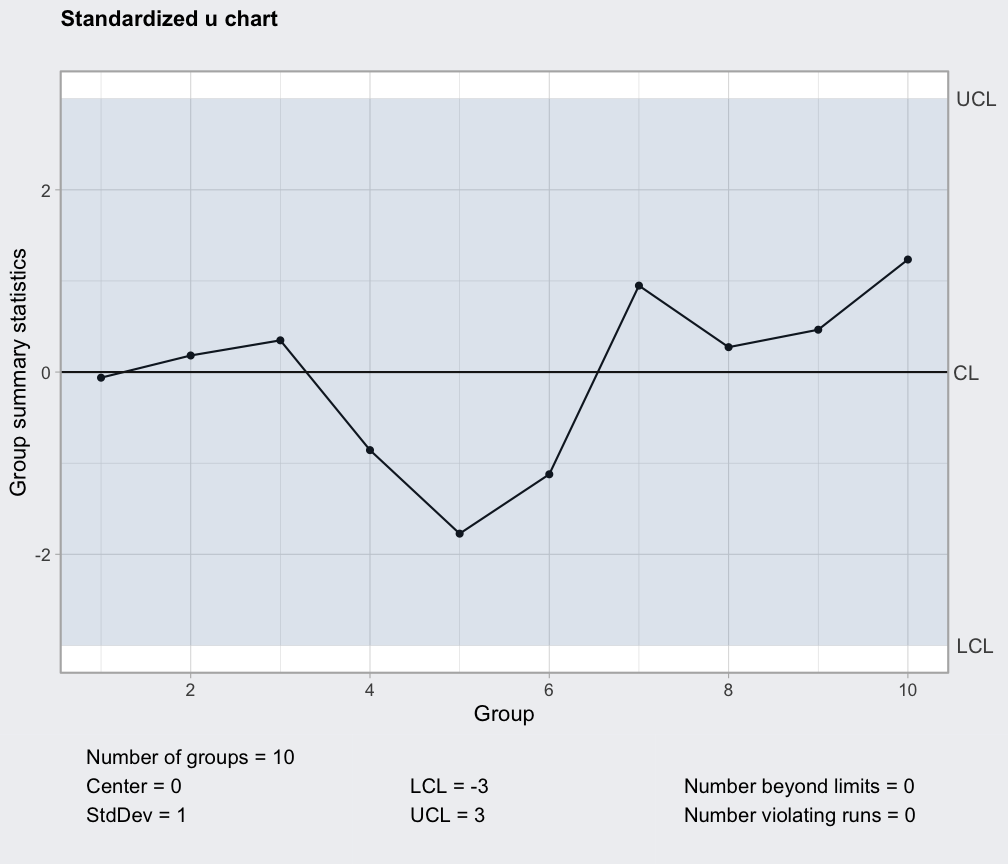 # standardized control chart
q = with(dyedcloth, qcc(x, sizes=size, type="u"))
z = (q$statistics - q$center)/sqrt(q$center/q$size)
plot(qcc(z, sizes = 1, type = "u", center = 0, std.dev = 1, limits = c(-3,3)),
title = "Standardized u chart")
#> Warning: 'std.dev' is not used when limits is given
# standardized control chart
q = with(dyedcloth, qcc(x, sizes=size, type="u"))
z = (q$statistics - q$center)/sqrt(q$center/q$size)
plot(qcc(z, sizes = 1, type = "u", center = 0, std.dev = 1, limits = c(-3,3)),
title = "Standardized u chart")
#> Warning: 'std.dev' is not used when limits is given
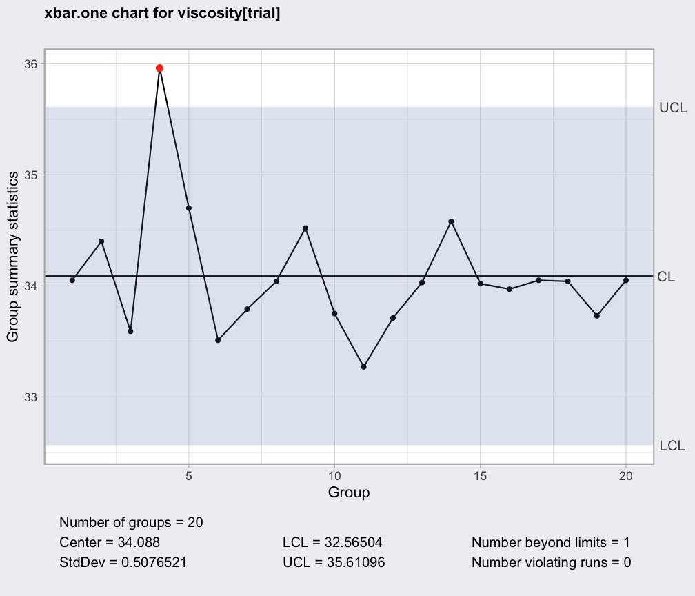 ##
## Continuous one-at-time data
##
data(viscosity)
q = with(viscosity,
qcc(viscosity[trial], type = "xbar.one"))
q
#> ── Quality Control Chart ─────────────────────────
#>
#> Chart type = xbar.one
#> Data (phase I) = viscosity[trial]
#> Number of groups = 20
#> Group sample size = 1
#> Center of group statistics = 34.088
#> Standard deviation = 0.5076521
#>
#> Control limits at nsigmas = 3
#> LCL UCL
#> 32.56504 35.61096
plot(q)
##
## Continuous one-at-time data
##
data(viscosity)
q = with(viscosity,
qcc(viscosity[trial], type = "xbar.one"))
q
#> ── Quality Control Chart ─────────────────────────
#>
#> Chart type = xbar.one
#> Data (phase I) = viscosity[trial]
#> Number of groups = 20
#> Group sample size = 1
#> Center of group statistics = 34.088
#> Standard deviation = 0.5076521
#>
#> Control limits at nsigmas = 3
#> LCL UCL
#> 32.56504 35.61096
plot(q)
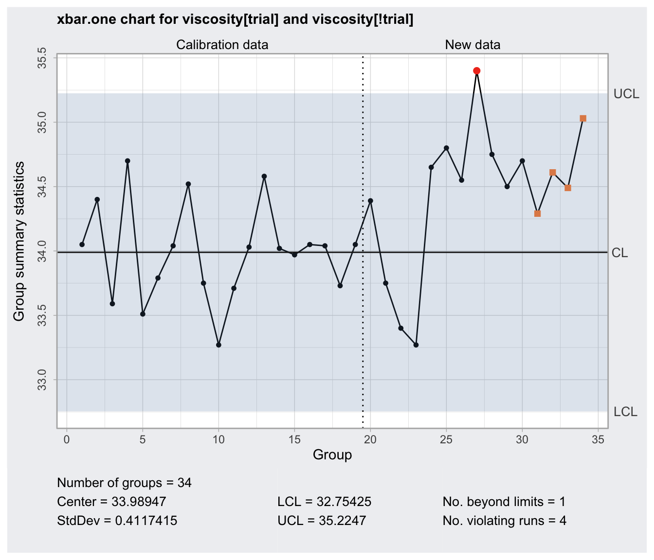
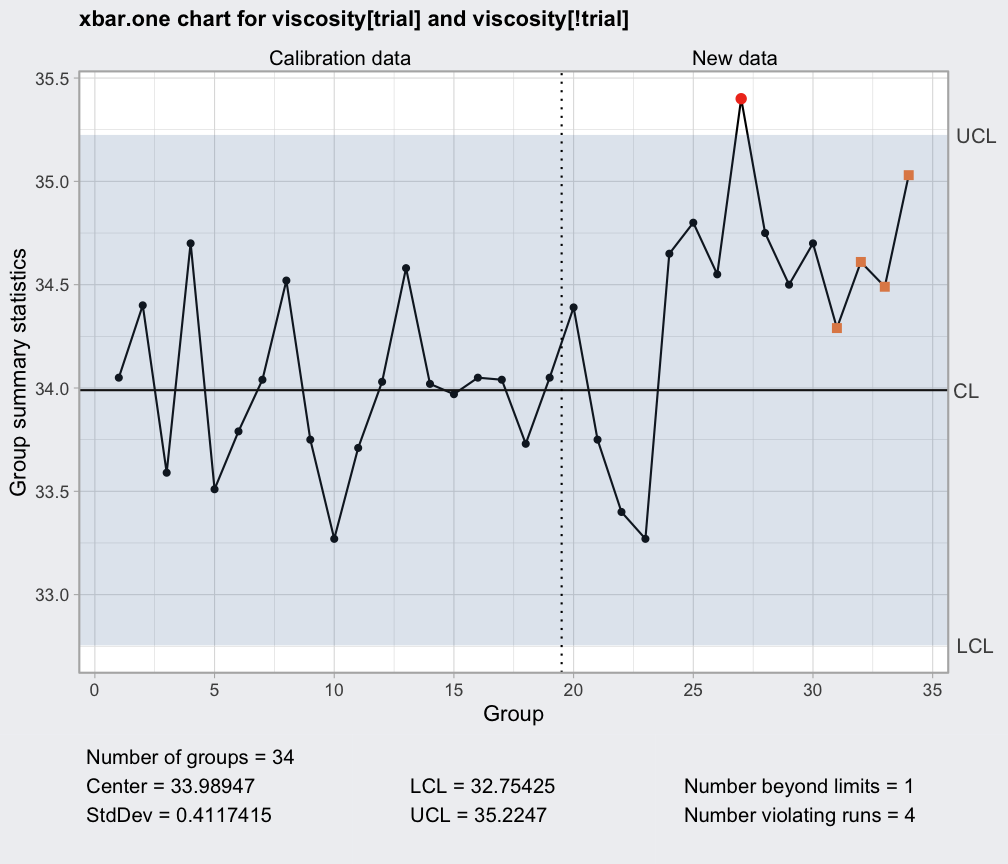 # batch 4 is out-of-control because of a process temperature controller
# failure; remove it and recompute
viscosity = viscosity[-4,]
plot(with(viscosity,
qcc(viscosity[trial], type = "xbar.one", newdata = viscosity[!trial])))
# batch 4 is out-of-control because of a process temperature controller
# failure; remove it and recompute
viscosity = viscosity[-4,]
plot(with(viscosity,
qcc(viscosity[trial], type = "xbar.one", newdata = viscosity[!trial])))