Introduction
qcc is a contributed R package for statistical
quality control charts which provides:
- Shewhart quality control charts for continuous, attribute and count data
- Cusum and EWMA charts
- Operating characteristic curves
- Process capability analysis
- Pareto chart and cause-and-effect chart
- Multivariate control charts.
This document gives a quick tour of qcc (version 3.0)
functionalities. Further details are provided in Scrucca (2004).
This vignette is written in R Markdown using the knitr package for production.
Shewhart charts
x-bar chart
data(pistonrings)
diameter <- qccGroups(data = pistonrings, diameter, sample)
head(diameter)
## [,1] [,2] [,3] [,4] [,5]
## 1 74.030 74.002 74.019 73.992 74.008
## 2 73.995 73.992 74.001 74.011 74.004
## 3 73.988 74.024 74.021 74.005 74.002
## 4 74.002 73.996 73.993 74.015 74.009
## 5 73.992 74.007 74.015 73.989 74.014
## 6 74.009 73.994 73.997 73.985 73.993
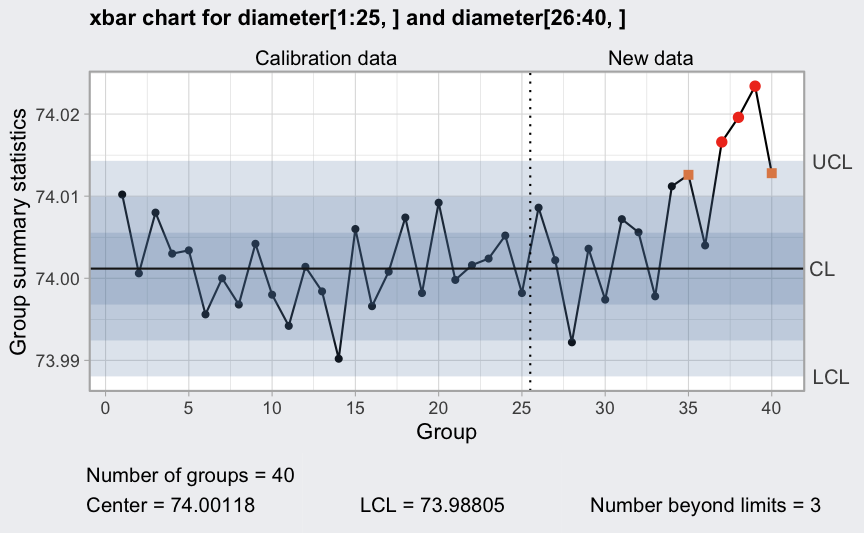
(q1 <- qcc(diameter[1:25,], type = "xbar",
newdata = diameter[26:40,]))
## ── Quality Control Chart ─────────────────────────
##
## Chart type = xbar
## Data (phase I) = diameter[1:25, ]
## Number of groups = 25
## Group sample size = 5
## Center of group statistics = 74.00118
## Standard deviation = 0.009785039
##
## New data (phase II) = diameter[26:40, ]
## Number of groups = 15
## Group sample size = 5
##
## Control limits at nsigmas = 3
## LCL UCL
## 73.98805 74.0143
plot(q1, fill = FALSE)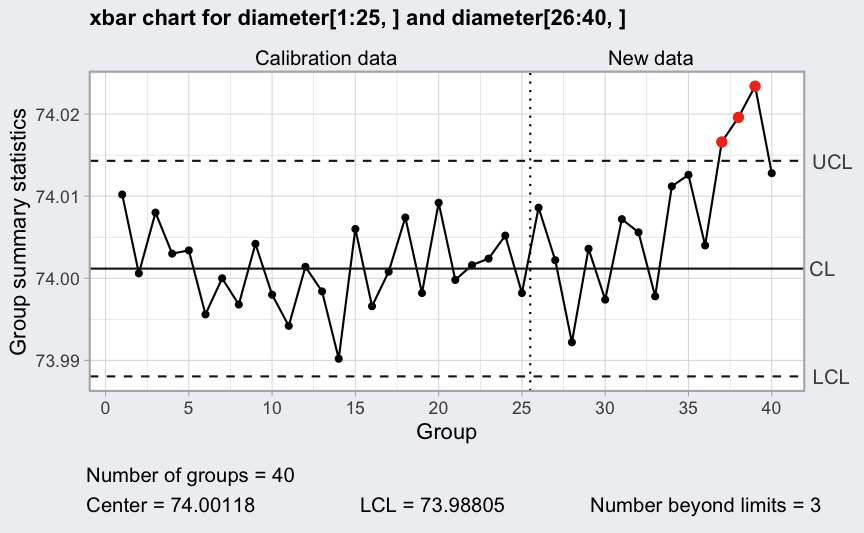
plot(q1, chart.all = FALSE)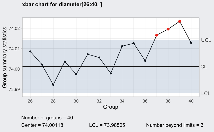
plot(q1, add.stats = FALSE)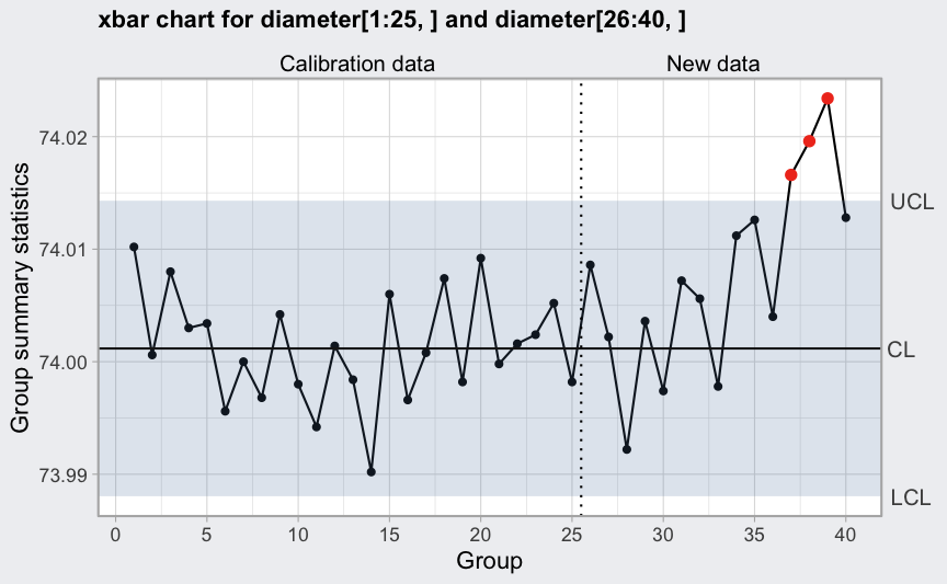
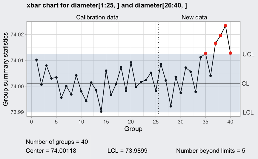
Western Electric rules:
plot(q1, fill = FALSE)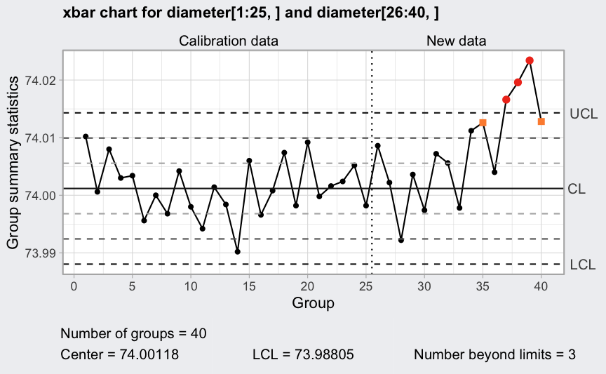
Specifying dates for rationale subgroups
In a Shewhart control chart the x-axis represents the rationale subgroups. This means that in the data collection process “subgroups or samples should be selected so that if assignable causes are present, the chance for differences between subgroups will be maximized, while the chance for differences due to these assignable causes within a subgroup will be minimized” (Montgomery, 2013, Sec. 5.3.4).
Typically, for control charts used in production processes the time order of production is a logical basis for rational subgroups. In this case a user may want to represent the date of production along the x-axis.
(dates <- seq(Sys.Date() - nrow(diameter)+1, Sys.Date(), by = 1))
##  [1] "2025-10-19" "2025-10-20" "2025-10-21" "2025-10-22" "2025-10-23"
##  [6] "2025-10-24" "2025-10-25" "2025-10-26" "2025-10-27" "2025-10-28"
## [11] "2025-10-29" "2025-10-30" "2025-10-31" "2025-11-01" "2025-11-02"
## [16] "2025-11-03" "2025-11-04" "2025-11-05" "2025-11-06" "2025-11-07"
## [21] "2025-11-08" "2025-11-09" "2025-11-10" "2025-11-11" "2025-11-12"
## [26] "2025-11-13" "2025-11-14" "2025-11-15" "2025-11-16" "2025-11-17"
## [31] "2025-11-18" "2025-11-19" "2025-11-20" "2025-11-21" "2025-11-22"
## [36] "2025-11-23" "2025-11-24" "2025-11-25" "2025-11-26" "2025-11-27"
q = qcc(diameter[1:25,], type = "xbar", newdata = diameter[26:40,])
plot(q, xtime = dates)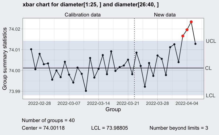
Further fine-tuning is also available as shown in the example below:
plot(q, xtime = dates, xlab = NULL, add.stats = FALSE) +
scale_x_date(date_breaks = "1 week", date_labels = "%d-%b")
## Scale for x is already present.
## Adding another scale for x, which will replace the existing scale.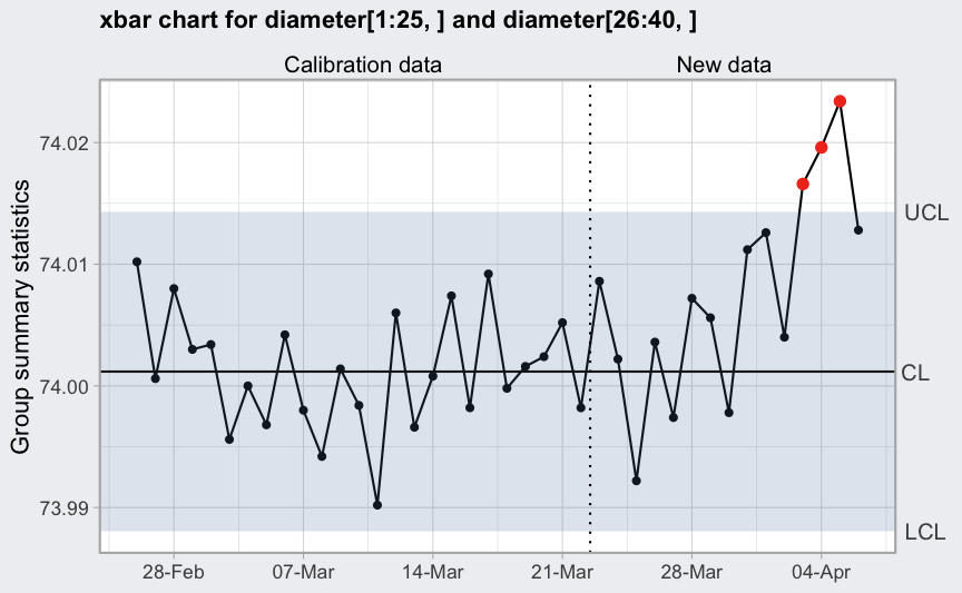 Note than we must remove the summary statistics at bottom
(
Note than we must remove the summary statistics at bottom
(add.stats = FALSE) in order to change the x-axis
settings.
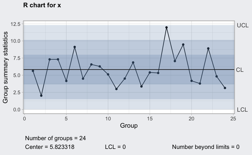
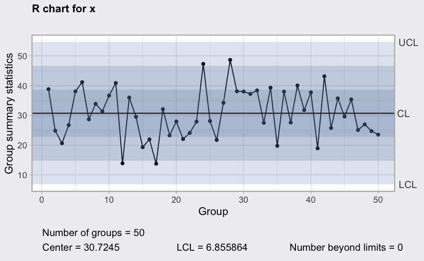
R chart
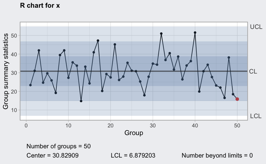
(q2 <- qcc(diameter[1:25,], type = "R"))
## ── Quality Control Chart ─────────────────────────
##
## Chart type                 = R
## Data (phase I)             = diameter[1:25, ]
## Number of groups           = 25
## Group sample size          = 5
## Center of group statistics = 0.02276
## Standard deviation         = 0.009785039
##
## Control limits at nsigmas  = 3
##  LCL        UCL
##    0 0.04812533
plot(q2)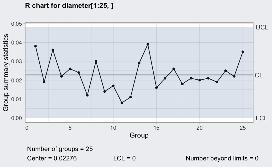
(q3 <- qcc(diameter[1:25,], type = "R", newdata = diameter[26:40,]))
## ── Quality Control Chart ─────────────────────────
##
## Chart type                 = R
## Data (phase I)             = diameter[1:25, ]
## Number of groups           = 25
## Group sample size          = 5
## Center of group statistics = 0.02276
## Standard deviation         = 0.009785039
##
## New data (phase II)        = diameter[26:40, ]
## Number of groups           = 15
## Group sample size          = 5
##
## Control limits at nsigmas  = 3
##  LCL        UCL
##    0 0.04812533
plot(q3)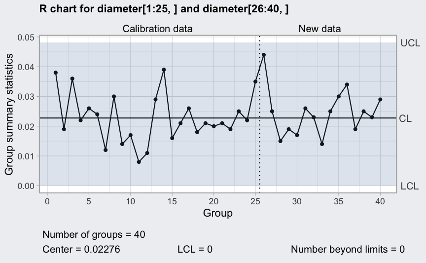
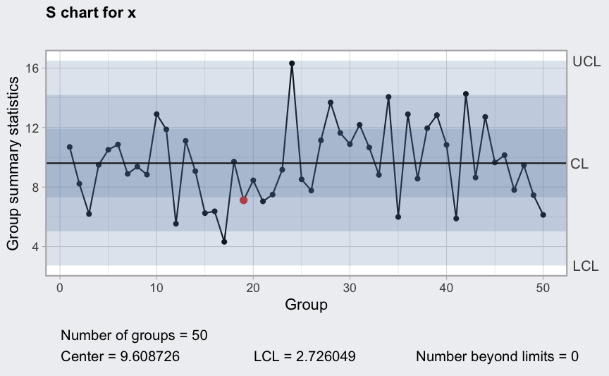
S chart
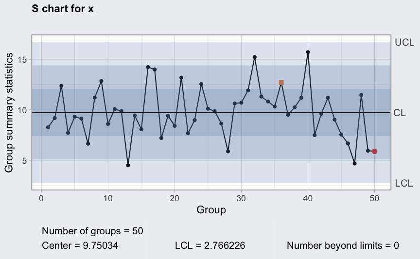
(q4 <- qcc(diameter[1:25,], type = "S"))
## ── Quality Control Chart ─────────────────────────
##
## Chart type                 = S
## Data (phase I)             = diameter[1:25, ]
## Number of groups           = 25
## Group sample size          = 5
## Center of group statistics = 0.009240037
## Standard deviation         = 0.009829977
##
## Control limits at nsigmas  = 3
##  LCL        UCL
##    0 0.01930242
plot(q4)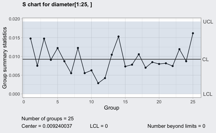
(q5 <- qcc(diameter[1:25,], type = "S", newdata = diameter[26:40,]))
## ── Quality Control Chart ─────────────────────────
##
## Chart type                 = S
## Data (phase I)             = diameter[1:25, ]
## Number of groups           = 25
## Group sample size          = 5
## Center of group statistics = 0.009240037
## Standard deviation         = 0.009829977
##
## New data (phase II)        = diameter[26:40, ]
## Number of groups           = 15
## Group sample size          = 5
##
## Control limits at nsigmas  = 3
##  LCL        UCL
##    0 0.01930242
plot(q5)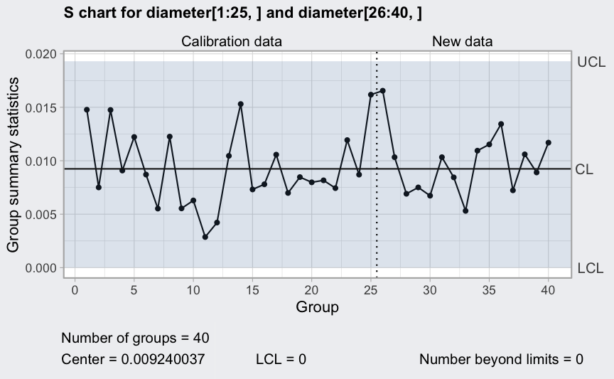
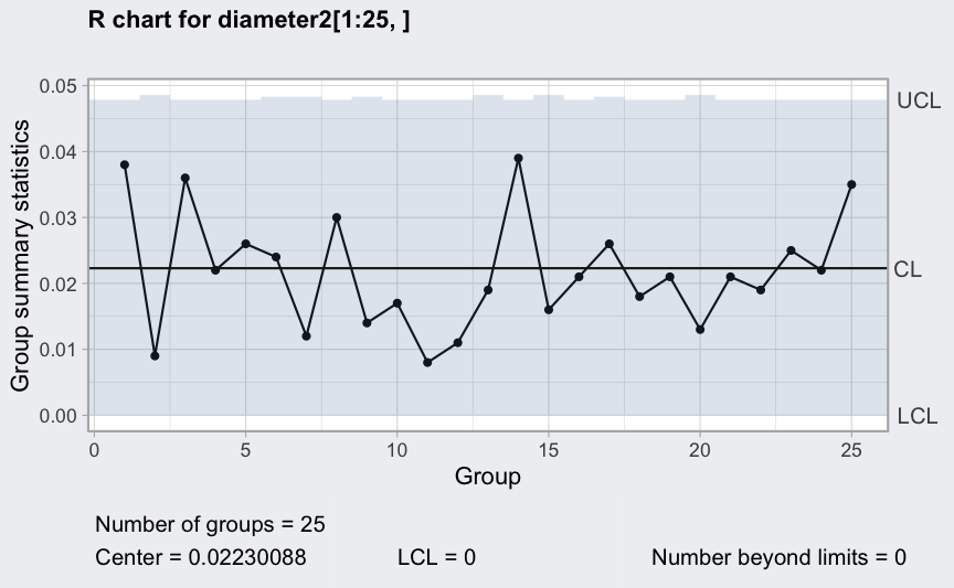
Variable control limits in control charts
out <- c(9, 10, 30, 35, 45, 64, 65, 74, 75, 85, 99, 100)
diameter2 <- qccGroups(data = pistonrings[-out,], diameter, sample)
plot(qcc(diameter2[1:25,], type = "xbar"))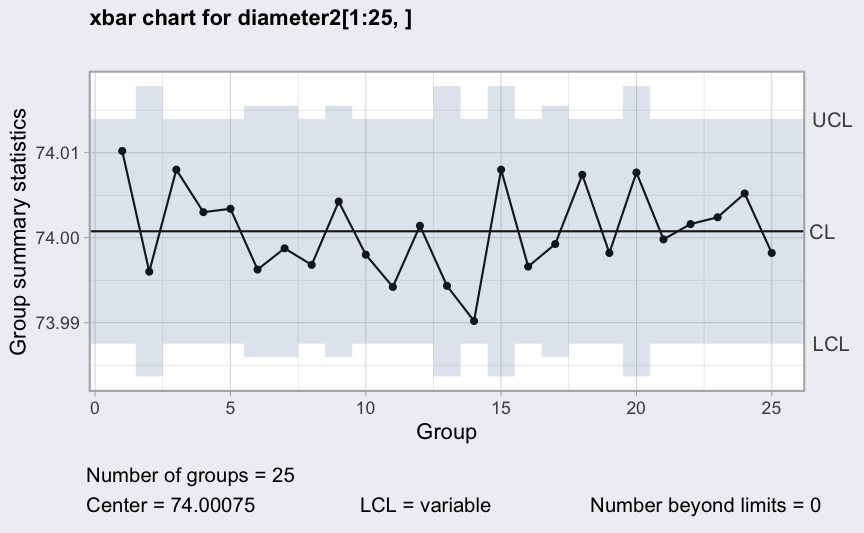
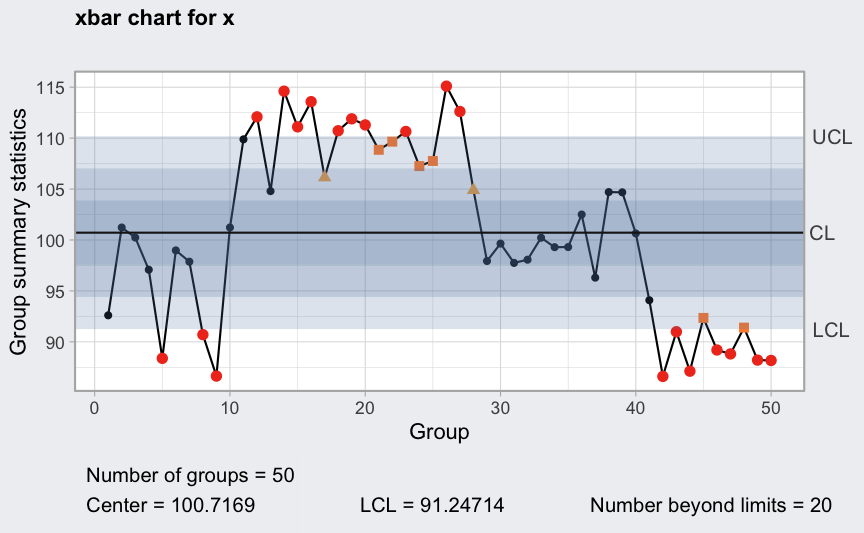
q = qcc(diameter2[1:25,], type = "xbar", rules = 1:4)
plot(qcc(diameter2[1:25,], type = "xbar", newdata = diameter2[26:40,], rules = 1:4))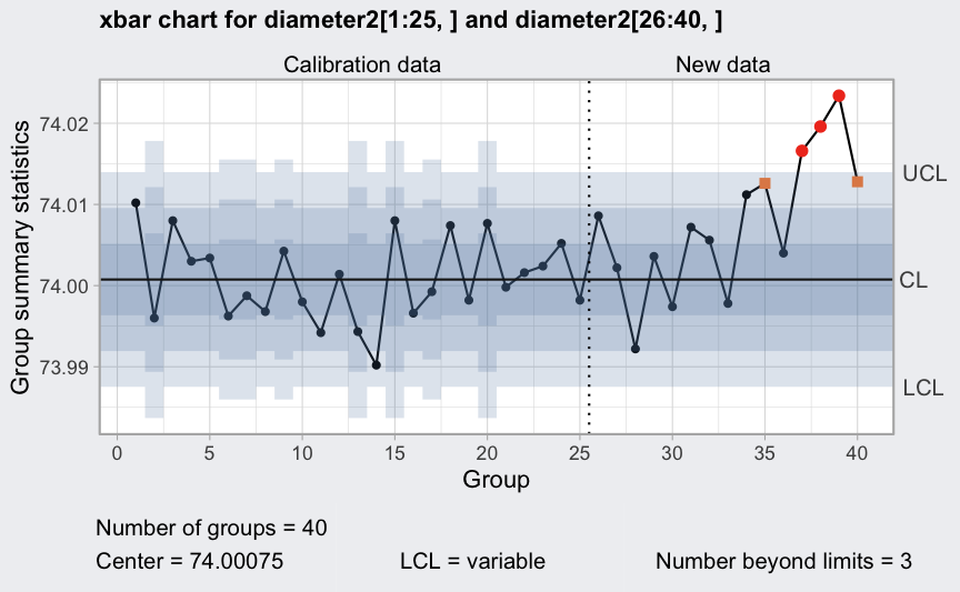
p and np charts
data(orangejuice)
(q = with(orangejuice, qcc(D[trial], sizes = size[trial], type = "p")))
## ── Quality Control Chart ─────────────────────────
##
## Chart type                 = p
## Data (phase I)             = D[trial]
## Number of groups           = 30
## Group sample size          = 50
## Center of group statistics = 0.2313333
## Standard deviation         = 0.05963526
##
## Control limits at nsigmas  = 3
##          LCL       UCL
##   0.05242755 0.4102391
##   0.05242755 0.4102391
## :
##   0.05242755 0.4102391
plot(q)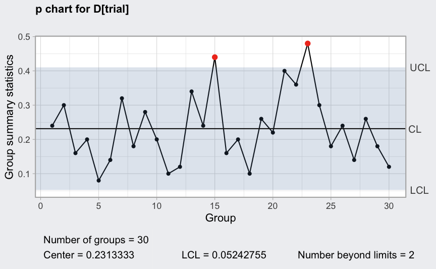
(q = with(orangejuice, qcc(D[trial], sizes = size[trial], type = "np")))
## ── Quality Control Chart ─────────────────────────
##
## Chart type                 = np
## Data (phase I)             = D[trial]
## Number of groups           = 30
## Group sample size          = 50
## Center of group statistics = 11.56667
## Standard deviation         = 2.981763
##
## Control limits at nsigmas  = 3
##       LCL      UCL
##  2.621377 20.51196
plot(q)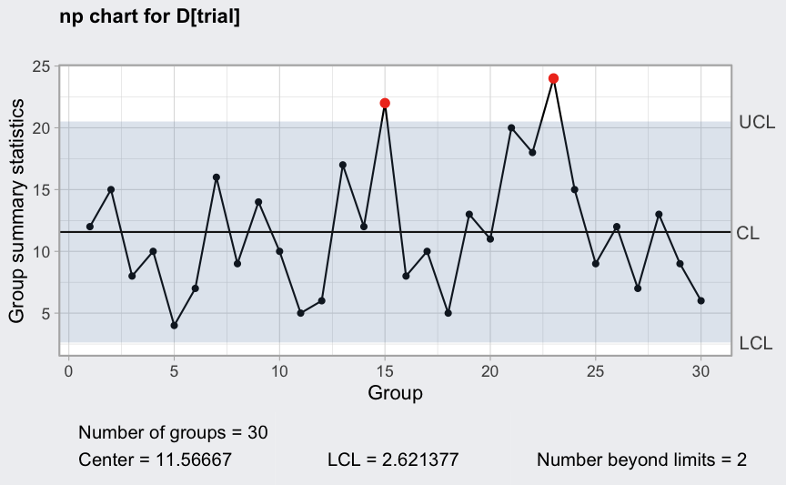
Remove out-of-control points (see help(orangejuice) for
the reasons):
inc <- setdiff(which(orangejuice$trial), c(15,23))
(q = with(orangejuice, qcc(D[inc], sizes = size[inc], type = "p",
                          newdata = D[!trial], newsizes = size[!trial])))
## ── Quality Control Chart ─────────────────────────
##
## Chart type                 = p
## Data (phase I)             = D[inc]
## Number of groups           = 28
## Group sample size          = 50
## Center of group statistics = 0.215
## Standard deviation         = 0.05809905
##
## New data (phase II)        = D[!trial]
## Number of groups           = 24
## Group sample size          = 50
##
## Control limits at nsigmas  = 3
##          LCL       UCL
##   0.04070284 0.3892972
##   0.04070284 0.3892972
## :
##   0.04070284 0.3892972
plot(q)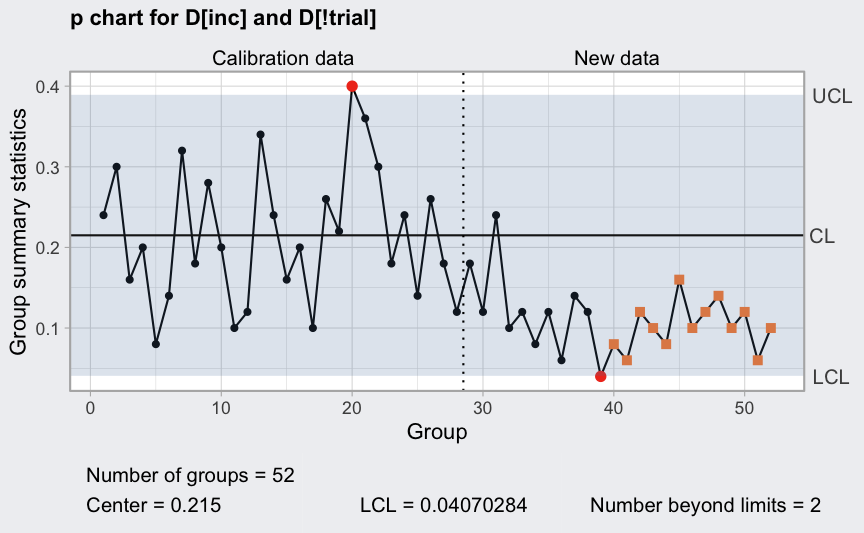
data(orangejuice2)
(q = with(orangejuice2, qcc(D[trial], sizes = size[trial], type = "p",
                            newdata = D[!trial], newsizes = size[!trial])))
## ── Quality Control Chart ─────────────────────────
##
## Chart type                 = p
## Data (phase I)             = D[trial]
## Number of groups           = 24
## Group sample size          = 50
## Center of group statistics = 0.1108333
## Standard deviation         = 0.04439579
##
## New data (phase II)        = D[!trial]
## Number of groups           = 40
## Group sample size          = 50
##
## Control limits at nsigmas  = 3
##   LCL       UCL
##     0 0.2440207
##     0 0.2440207
## :
##     0 0.2440207
plot(q)
c and u charts
data(circuit)
(q = with(circuit, qcc(x[trial], sizes = size[trial], type = "c")))
## ── Quality Control Chart ─────────────────────────
##
## Chart type                 = c
## Data (phase I)             = x[trial]
## Number of groups           = 26
## Group sample size          = 100
## Center of group statistics = 19.84615
## Standard deviation         = 4.454902
##
## Control limits at nsigmas  = 3
##       LCL      UCL
##  6.481447 33.21086
plot(q)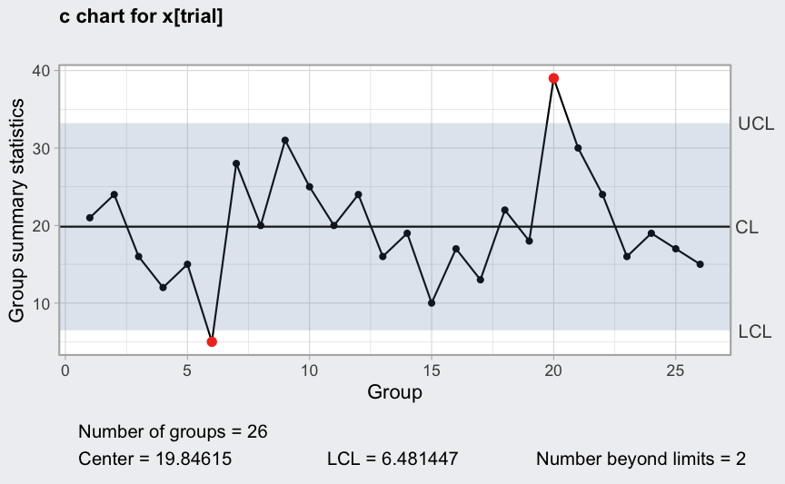
Remove out-of-control points (see help(circuit) for the
reasons)
inc <- setdiff(which(circuit$trial), c(6,20))
(q = with(circuit, qcc(x[inc], sizes = size[inc], type = "c", labels = inc,
                       newdata = x[!trial], newsizes = size[!trial],
                       newlabels = which(!trial))))
## ── Quality Control Chart ─────────────────────────
##
## Chart type                 = c
## Data (phase I)             = x[inc]
## Number of groups           = 24
## Group sample size          = 100
## Center of group statistics = 19.66667
## Standard deviation         = 4.434712
##
## New data (phase II)        = x[!trial]
## Number of groups           = 20
## Group sample size          = 100
##
## Control limits at nsigmas  = 3
##       LCL     UCL
##  6.362532 32.9708
plot(q)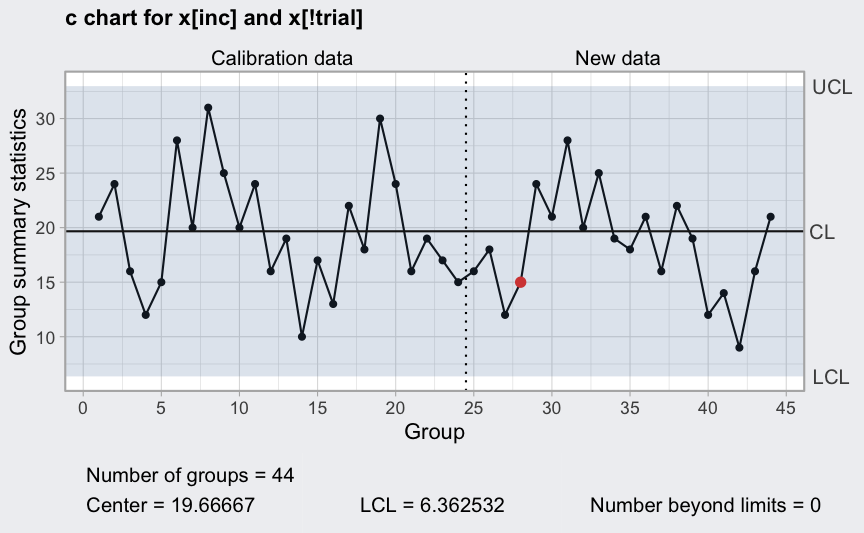
(q = with(circuit, qcc(x[inc], sizes = size[inc], type = "u", labels = inc,
                       newdata = x[!trial], newsizes = size[!trial],
                       newlabels = which(!trial))))
## ── Quality Control Chart ─────────────────────────
##
## Chart type                 = u
## Data (phase I)             = x[inc]
## Number of groups           = 24
## Group sample size          = 100
## Center of group statistics = 0.1966667
## Standard deviation         = 0.4434712
##
## New data (phase II)        = x[!trial]
## Number of groups           = 20
## Group sample size          = 100
##
## Control limits at nsigmas  = 3
##         LCL      UCL
##  0.06362532 0.329708
plot(q)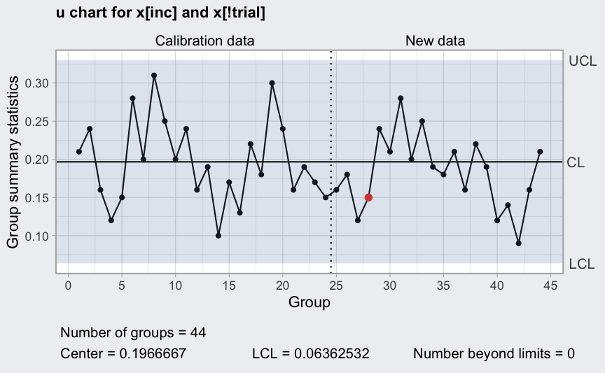
data(pcmanufact)
(q = with(pcmanufact, qcc(x, sizes = size, type = "u")))
## ── Quality Control Chart ─────────────────────────
##
## Chart type                 = u
## Data (phase I)             = x
## Number of groups           = 20
## Group sample size          = 5
## Center of group statistics = 1.93
## Standard deviation         = 1.389244
##
## Control limits at nsigmas  = 3
##         LCL      UCL
##  0.06613305 3.793867
plot(q)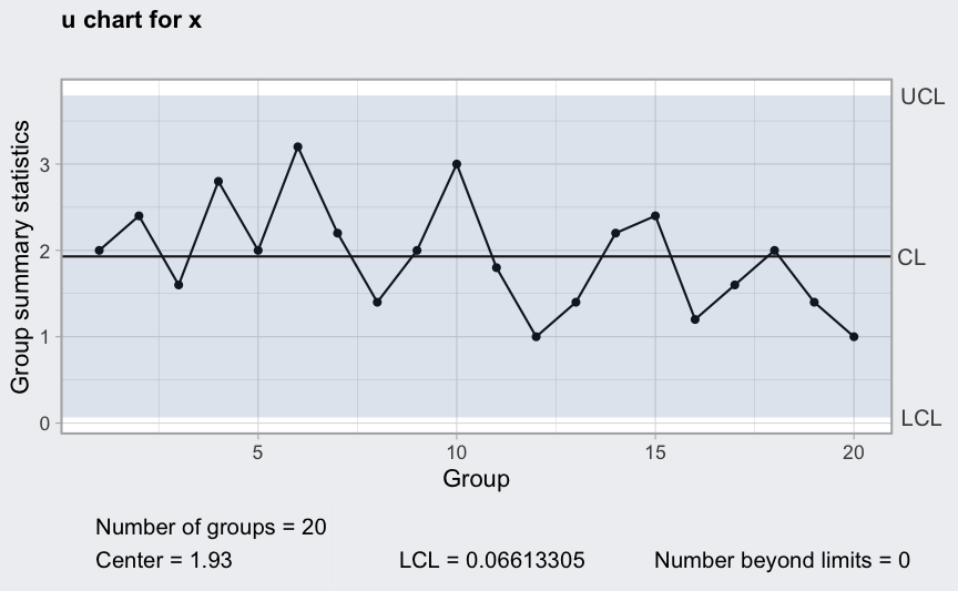
Continuous one-at-time data
data(viscosity)
(q = with(viscosity, qcc(viscosity[trial], type = "xbar.one")))
## ── Quality Control Chart ─────────────────────────
##
## Chart type                 = xbar.one
## Data (phase I)             = viscosity[trial]
## Number of groups           = 20
## Group sample size          = 1
## Center of group statistics = 34.088
## Standard deviation         = 0.5076521
##
## Control limits at nsigmas  = 3
##       LCL      UCL
##  32.56504 35.61096
plot(q)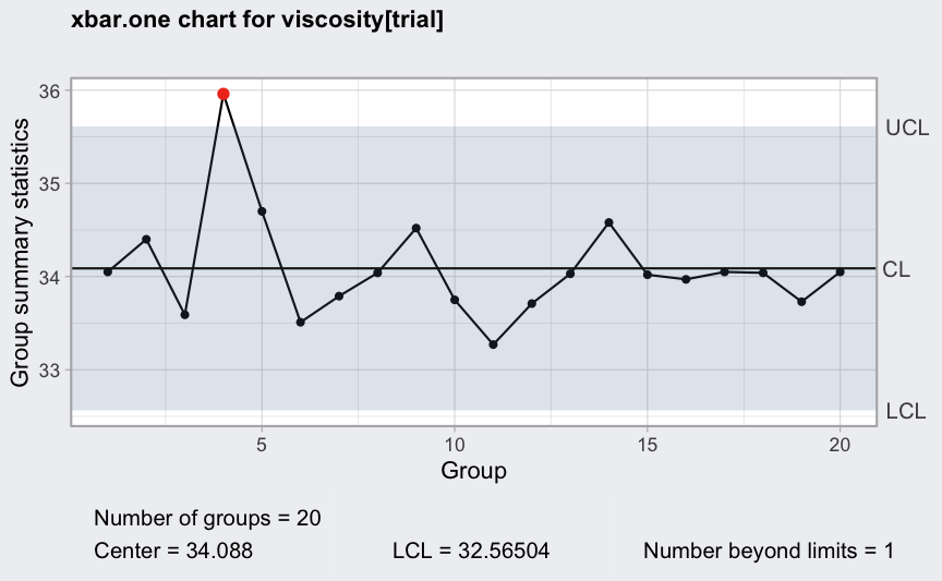
(q = with(viscosity, qcc(viscosity[trial], type = "xbar.one", std.dev = "SD")))
## ── Quality Control Chart ─────────────────────────
##
## Chart type                 = xbar.one
## Data (phase I)             = viscosity[trial]
## Number of groups           = 20
## Group sample size          = 1
## Center of group statistics = 34.088
## Standard deviation         = 0.5769854
##
## Control limits at nsigmas  = 3
##       LCL      UCL
##  32.35704 35.81896
plot(q)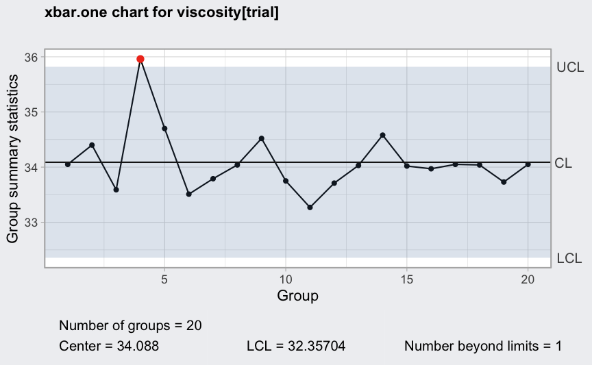
# batch 4 is out-of-control because of a process temperature controller
# failure; remove it and recompute
viscosity <- viscosity[-4,]
(q = with(viscosity, qcc(viscosity[trial], type = "xbar.one",
                         newdata = viscosity[!trial],
                         rules = 1:4)))
## ── Quality Control Chart ─────────────────────────
##
## Chart type                 = xbar.one
## Data (phase I)             = viscosity[trial]
## Number of groups           = 19
## Group sample size          = 1
## Center of group statistics = 33.98947
## Standard deviation         = 0.4117415
##
## New data (phase II)        = viscosity[!trial]
## Number of groups           = 15
## Group sample size          = 1
##
## Control limits at nsigmas  = 3
##       LCL     UCL
##  32.75425 35.2247
plot(q)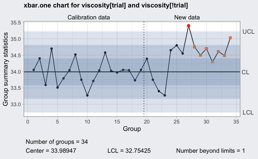
Standardized p chart
In this example we show how to extend the package by defining a new
control chart, i.e. a standardized p chart
(type = "p.std").
Function to compute group statistics and center:
stats.p.std <- function(data, sizes)
{
  data <- as.vector(data)
  sizes <- as.vector(sizes)
  pbar <- sum(data)/sum(sizes)
  z <- (data/sizes - pbar)/sqrt(pbar*(1-pbar)/sizes)
  list(statistics = z, center = 0)
}
Function to compute within-group standard deviation:
sd.p.std <- function(data, sizes, ...) { return(1) }Function to compute control limits based on normal approximation:
limits.p.std <- function(center, std.dev, sizes, nsigmas = NULL, conf = NULL)
{
  if(is.null(conf))
    { lcl <- -nsigmas
      ucl <- +nsigmas
  } else
    { if(conf > 0 & conf < 1)
        { nsigmas <- qnorm(1 - (1 - conf)/2)
          lcl <- -nsigmas
          ucl <- +nsigmas }
      else stop("invalid 'conf' argument.")
  }
  limits <- matrix(c(lcl, ucl), ncol = 2)
  rownames(limits) <- rep("", length = nrow(limits))
  colnames(limits) <- c("LCL", "UCL")
  return(limits)
}
Example with simulated data:
# set unequal sample sizes
n <- c(rep(50,5), rep(100,5), rep(25, 5))
# generate randomly the number of successes
x <- rbinom(length(n), n, 0.2)
# plot the control chart with variable limits
(q = qcc(x, type = "p", size = n))
## ── Quality Control Chart ─────────────────────────
##
## Chart type                 = p
## Data (phase I)             = x
## Number of groups           = 15
## Group sample sizes         =
##   sizes  25 50 100
##   counts  5  5   5
## Center of group statistics = 0.2148571
## Standard deviation         = 0.05808503 0.05808503 0.05808503 ...
##
## Control limits at nsigmas  = 3
##          LCL       UCL
##   0.04060204 0.3891122
##   0.04060204 0.3891122
## :
##   0.00000000 0.4612911
plot(q)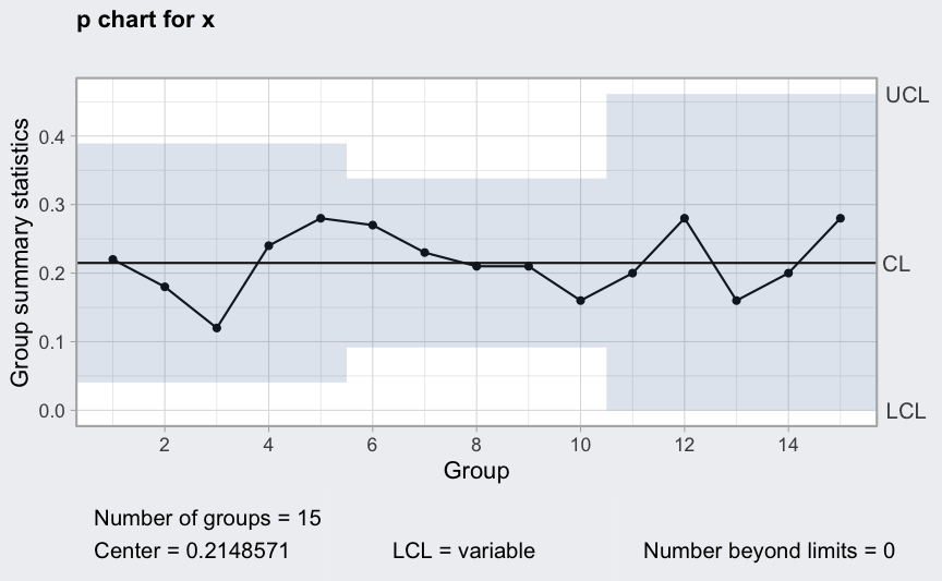
# plot the standardized control chart
(q = qcc(x, type = "p.std", size = n))
## ── Quality Control Chart ─────────────────────────
##
## Chart type                 = p.std
## Data (phase I)             = x
## Number of groups           = 15
## Group sample sizes         =
##   sizes  25 50 100
##   counts  5  5   5
## Center of group statistics = 0
## Standard deviation         = 1
##
## Control limits at nsigmas  = 3
##  LCL UCL
##   -3   3
plot(q)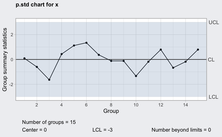
Operating Characteristic Curves
An operating characteristic curve graphically provides information
about the probability of not detecting a shift in the process. The
function ocCurves() is a generic function which calls the
proper function depending on the type of input 'qcc'
object.
data(pistonrings)
diameter <- qccGroups(data = pistonrings, diameter, sample)
q <- qcc(diameter, type = "xbar", nsigmas = 3)
(beta <- ocCurves(q))
## ── Operating Characteristic Curves ───────────────
##
## Chart type:  xbar
##
## Prob. type II error (beta):
##               sample size
## shift (StdDev)      1      5     10     15     20
##            0.0 0.9973 0.9973 0.9973 0.9973 0.9973
##            0.1 0.9972 0.9966 0.9959 0.9952 0.9944
##            0.2 0.9968 0.9944 0.9909 0.9869 0.9823
##            :
##            4.9 0.0287 0.0000 0.0000 0.0000 0.0000
##            5.0 0.0228 0.0000 0.0000 0.0000 0.0000
##
## Average run length (ARL):
##               sample size
## shift (StdDev)   1   5  10  15  20
##            0.0 370 370 370 370 370
##            0.1 353 296 244 206 178
##            0.2 308 178 110  76  57
##            :
##            4.9   1   1   1   1   1
##            5.0   1   1   1   1   1
plot(beta)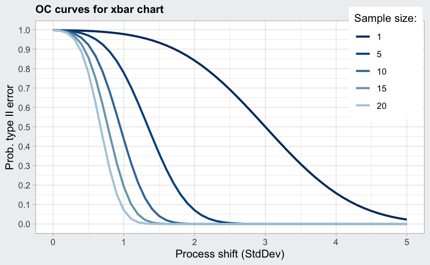
plot(beta, what = "ARL")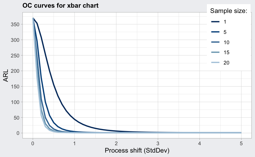
data(orangejuice)
q <- with(orangejuice, qcc(D[trial], sizes = size[trial], type = "p"))
(beta <- ocCurves(q))
## ── Operating Characteristic Curves ───────────────
##
## Chart type:  p
##
## Prob. type II error (beta):
##
## fraction nonconforming   beta
##                   0.00 0.0000
##                   0.01 0.0894
##                   0.02 0.2642
##                   :
##                   0.99 0.0000
##                   1.00 0.0000
##
## Average run length (ARL):
##
## fraction nonconforming ARL
##                   0.00   1
##                   0.01   1
##                   0.02   1
##                   :
##                   0.99   1
##                   1.00   1
plot(beta)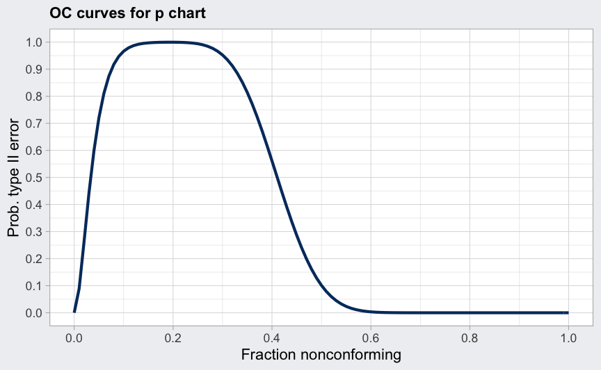
plot(beta, what = "ARL")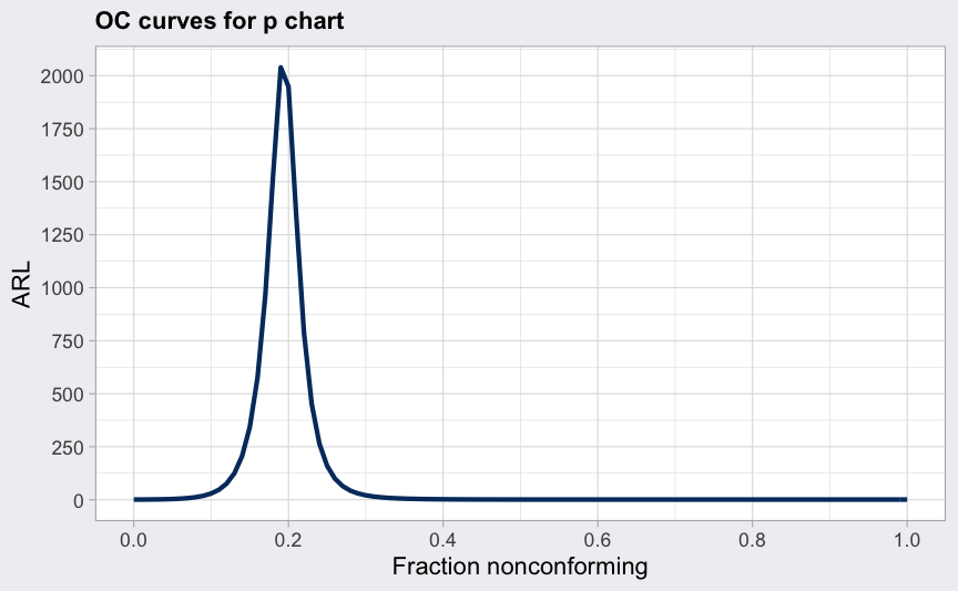
data(circuit)
q <- with(circuit, qcc(x[trial], sizes = size[trial], type = "c"))
(beta <- ocCurves(q))
## ── Operating Characteristic Curves ───────────────
##
## Chart type:  c
##
## Prob. type II error (beta):
##
## average nonconforming   beta
##                 0.00  0.0000
##                 1.00  0.0006
##                 2.00  0.0166
##                 :
##                 64.00 0.0000
##                 65.00 0.0000
##
## Average run length (ARL):
##
## average nonconforming ARL
##                 0.00    1
##                 1.00    1
##                 2.00    1
##                 :
##                 64.00   1
##                 65.00   1
plot(beta)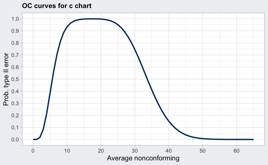
plot(beta, what = "ARL")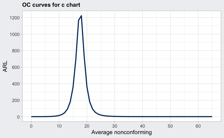
Cusum chart
data(pistonrings)
diameter <- qccGroups(diameter, sample, data = pistonrings)

(q = cusum(diameter[1:25,], decision.interval = 4, se.shift = 1))
## ── Cusum Chart ───────────────────────────────────
##
## Data (phase I)             = diameter[1:25, ]
## Number of groups           = 25
## Group sample size          = 5
## Center of group statistics = 74.00118
## Standard deviation         = 0.009785039
##
## Decision interval (StdErr) = 4
## Shift detection   (StdErr) = 1
plot(q)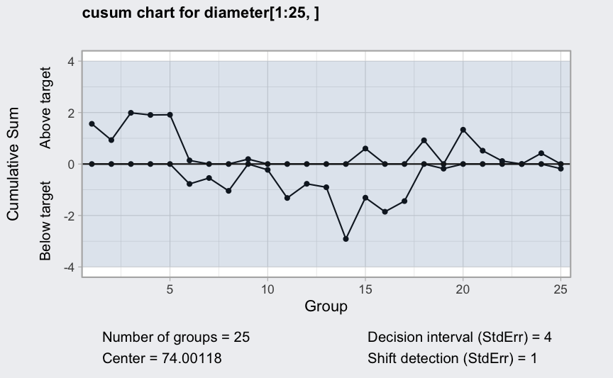
(q <- cusum(diameter[1:25,], newdata = diameter[26:40,]))
## ── Cusum Chart ───────────────────────────────────
##
## Data (phase I)             = diameter[1:25, ]
## Number of groups           = 25
## Group sample size          = 5
## Center of group statistics = 74.00118
## Standard deviation         = 0.009785039
##
## New data (phase II)        = diameter[26:40, ]
## Number of groups           = 15
## Group sample size          = 5
##
## Decision interval (StdErr) = 5
## Shift detection   (StdErr) = 1
plot(q)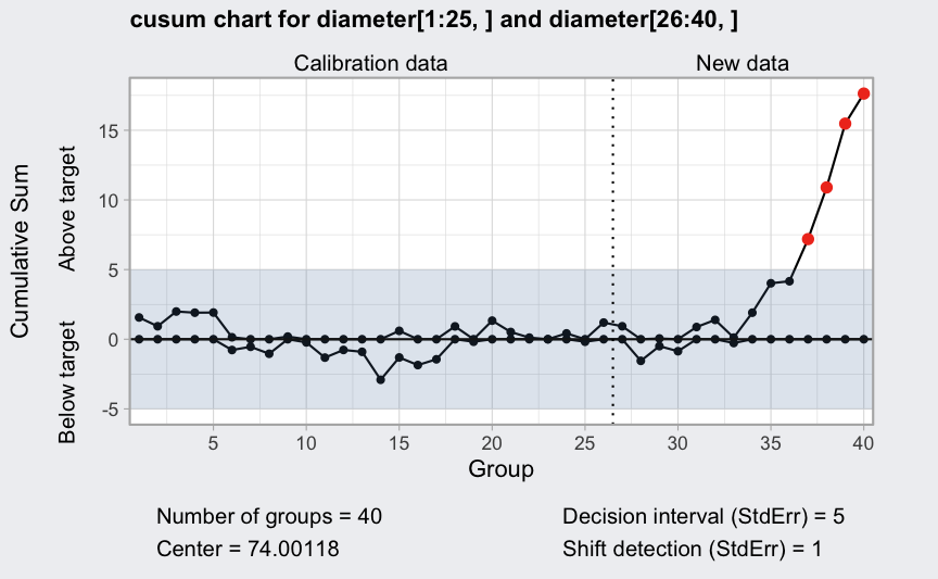
plot(q, chart.all = FALSE)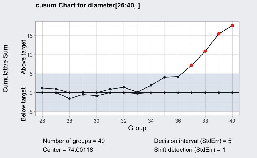
plot(q, xtime = seq(Sys.Date() - nrow(diameter)+1, Sys.Date(), by = 1),
     add.stats = FALSE) +
  scale_x_date(date_breaks = "4 days", date_labels = "%d-%b")
## Scale for x is already present.
## Adding another scale for x, which will replace the existing scale.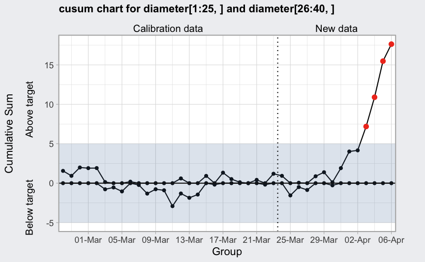
EWMA
data(pistonrings)
diameter <- qccGroups(data = pistonrings, diameter, sample)

(q = ewma(diameter[1:25,], lambda = 0.2, nsigmas = 3))
## ── EWMA Chart ────────────────────────────────────
##
## Data (phase I)             = diameter[1:25, ]
## Number of groups           = 25
## Group sample size          = 5
## Center of group statistics = 74.00118
## Standard deviation         = 0.009785039
##
## Smoothing parameter        = 0.2
## Control limits at nsigmas  = 3
##         LCL      UCL
## 1  73.99855 74.00380
## 2  73.99781 74.00454
## :
## 25 73.99680 74.00555
plot(q)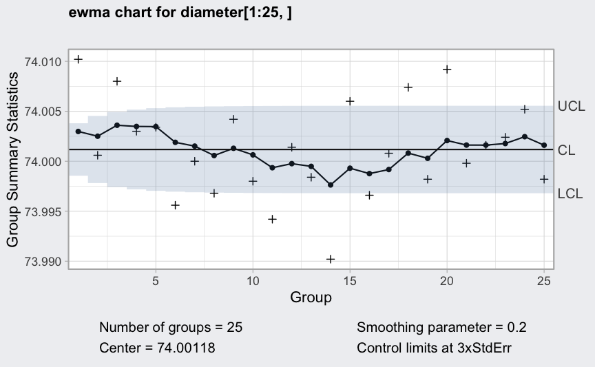
(q = ewma(diameter[1:25,], lambda = 0.2, nsigmas = 2.7, newdata = diameter[26:40,]))
## ── EWMA Chart ────────────────────────────────────
##
## Data (phase I)             = diameter[1:25, ]
## Number of groups           = 25
## Group sample size          = 5
## Center of group statistics = 74.00118
## Standard deviation         = 0.009785039
##
## New data (phase II)        = diameter[26:40, ]
## Number of groups           = 15
## Group sample size          = 5
##
## Smoothing parameter        = 0.2
## Control limits at nsigmas  = 2.7
##         LCL      UCL
## 1  73.99881 74.00354
## 2  73.99815 74.00420
## :
## 40 73.99724 74.00511
plot(q)
plot(q, xtime = seq(Sys.Date() - nrow(diameter)+1, Sys.Date(), by = 1),
     add.stats = FALSE) +
  scale_x_date(date_breaks = "4 days", date_labels = "%d-%b")
## Scale for x is already present.
## Adding another scale for x, which will replace the existing scale.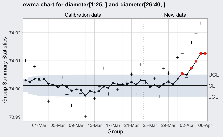
data(viscosity)
(q = with(viscosity,
          ewma(viscosity[trial], lambda = 0.2, nsigmas = 2.7,
               newdata = viscosity[!trial])))
## ── EWMA Chart ────────────────────────────────────
##
## Data (phase I)             = viscosity[trial]
## Number of groups           = 20
## Group sample size          = 1
## Center of group statistics = 34.088
## Standard deviation         = 0.5076521
##
## New data (phase II)        = viscosity[!trial]
## Number of groups           = 15
## Group sample size          = 1
##
## Smoothing parameter        = 0.2
## Control limits at nsigmas  = 2.7
##            LCL      UCL
## [1,]  33.81387 34.36213
## [2,]  33.73694 34.43906
## :
## [35,] 33.63111 34.54489
plot(q)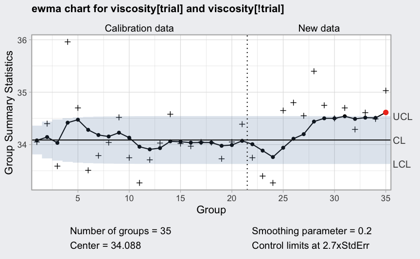
Process capability analysis
data(pistonrings)
diameter <- qccGroups(data = pistonrings, diameter, sample)

q <- qcc(diameter[1:25,], type = "xbar", nsigmas = 3)

(pc = processCapability(q, spec.limits = c(73.95,74.05)))
## ── Process Capability Analysis ───────────────────
##
## Number of obs = 125          Target = 74
## Center        = 74.00118     LSL    = 73.95
## StdDev        = 0.009785039  USL    = 74.05
##
## Capability indices  Value  2.5%  97.5%
##               Cp     1.70  1.49   1.91
##               Cp_l   1.74  1.55   1.93
##               Cp_u   1.66  1.48   1.84
##               Cp_k   1.66  1.45   1.88
##               Cpm    1.69  1.48   1.90
##
## Exp<LSL 0%    Obs<LSL 0%
## Exp>USL 0%    Obs>USL 0%
plot(pc)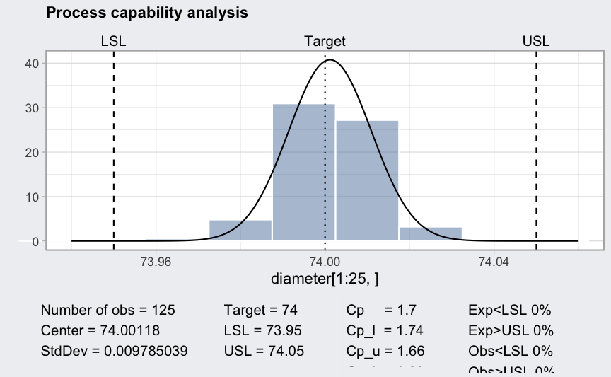
(pc = processCapability(q, spec.limits = c(73.95,74.05), target = 74.02))
## ── Process Capability Analysis ───────────────────
##
## Number of obs = 125          Target = 74.02
## Center        = 74.00118     LSL    = 73.95
## StdDev        = 0.009785039  USL    = 74.05
##
## Capability indices  Value   2.5%  97.5%
##               Cp    1.703  1.491  1.915
##               Cp_l  1.743  1.555  1.932
##               Cp_u  1.663  1.483  1.844
##               Cp_k  1.663  1.448  1.878
##               Cpm   0.786  0.656  0.915
##
## Exp<LSL 0%    Obs<LSL 0%
## Exp>USL 0%    Obs>USL 0%
plot(pc)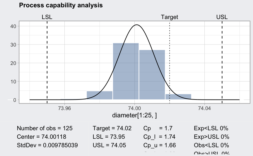
(pc = processCapability(q, spec.limits = c(73.99,74.01)))
## ── Process Capability Analysis ───────────────────
##
## Number of obs = 125          Target = 74
## Center        = 74.00118     LSL    = 73.99
## StdDev        = 0.009785039  USL    = 74.01
##
## Capability indices  Value   2.5%  97.5%
##               Cp    0.341  0.298  0.383
##               Cp_l  0.381  0.318  0.444
##               Cp_u  0.301  0.242  0.359
##               Cp_k  0.301  0.231  0.370
##               Cpm   0.338  0.296  0.380
##
## Exp<LSL 13%   Obs<LSL 12%
## Exp>USL 18%   Obs>USL 16%
plot(pc)
(pc = processCapability(q, spec.limits = c(73.99, 74.1)))
## ── Process Capability Analysis ───────────────────
##
## Number of obs = 125          Target = 74.045
## Center        = 74.00118     LSL    = 73.99
## StdDev        = 0.009785039  USL    = 74.1
##
## Capability indices  Value   2.5%  97.5%
##               Cp    1.874  1.641  2.106
##               Cp_l  0.381  0.318  0.444
##               Cp_u  3.367  3.011  3.722
##               Cp_k  0.381  0.305  0.456
##               Cpm   0.408  0.338  0.479
##
## Exp<LSL 13%   Obs<LSL 12%
## Exp>USL 0%    Obs>USL 0%
plot(pc)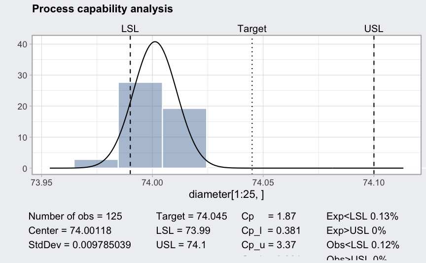
Multivariate Quality Control Charts
Multivariate subgrouped data from Ryan (2011, Table 9.2) with variables, samples, and sample size for each sample:
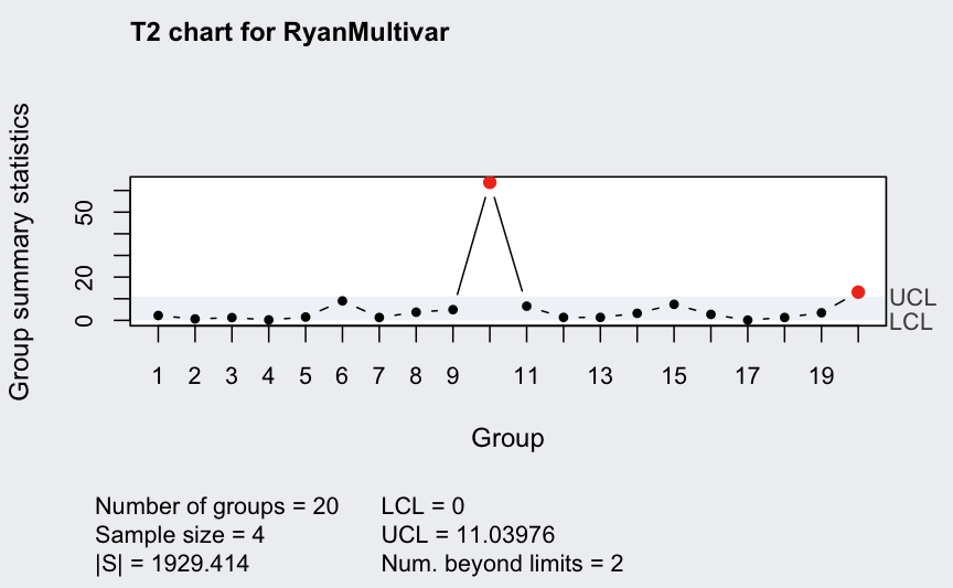
## ── Multivariate Quality Control Chart ────────────
##
## Chart type                 = T2
## Data (phase I)             = RyanMultivar
## Number of groups           = 20
## Group sample size          = 4
## Center =
##      X1      X2
## 60.3750 18.4875
## Covariance matrix =
##          X1        X2
## X1 222.0333 103.11667
## X2 103.1167  56.57917
## |S| = 1929.414
##
## Control limits:
##  LCL      UCL
##    0 11.03976

ellipseChart(q)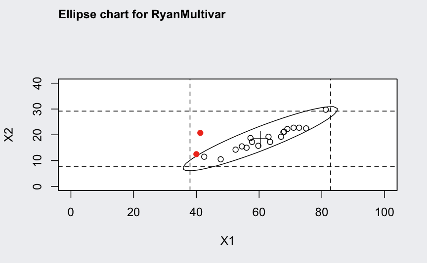
ellipseChart(q, show.id = TRUE)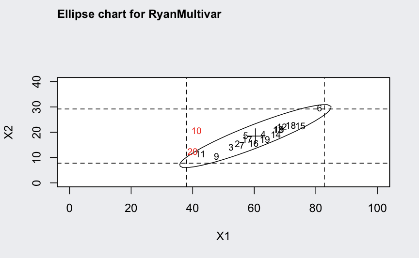
q <- mqcc(RyanMultivar, type = "T2", pred.limits = TRUE)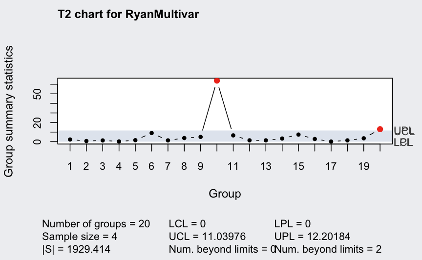
Ryan (2011) discussed Xbar-charts for single variables computed adjusting the confidence level of the chart:
with(RyanMultivar,
     qcc(X1, type = "xbar", confidence.level = q$confidence.level^(1/2)))
## ── Quality Control Chart ─────────────────────────
##
## Chart type                 = xbar
## Data (phase I)             = X1
## Number of groups           = 20
## Group sample size          = 4
## Center of group statistics = 60.375
## Standard deviation         = 14.93443
##
## Control limits at nsigmas  = 2.999977
##       LCL      UCL
##  37.97352 82.77648

with(RyanMultivar,
     qcc(X2, type = "xbar", confidence.level = q$confidence.level^(1/2)))
## ── Quality Control Chart ─────────────────────────
##
## Chart type                 = xbar
## Data (phase I)             = X2
## Number of groups           = 20
## Group sample size          = 4
## Center of group statistics = 18.4875
## Standard deviation         = 7.139388
##
## Control limits at nsigmas  = 2.999977
##     LCL     UCL
##  7.7785 29.1965
Generate new “in control” data:
Xnew <- list(X1 = matrix(NA, 10, 4), X2 =  matrix(NA, 10, 4))
for(i in 1:4)
   { x <- MASS::mvrnorm(10, mu = q$center, Sigma = q$cov)
     Xnew$X1[,i] <- x[,1]
     Xnew$X2[,i] <- x[,2]
   }
(q <- mqcc(RyanMultivar, type = "T2", newdata = Xnew, pred.limits = TRUE))
## ── Multivariate Quality Control Chart ────────────
##
## Chart type                 = T2
## Data (phase I)             = RyanMultivar
## Number of groups           = 20
## Group sample size          = 4
## Center =
##      X1      X2
## 60.3750 18.4875
## Covariance matrix =
##          X1        X2
## X1 222.0333 103.11667
## X2 103.1167  56.57917
## |S| = 1929.414
##
## New data (phase II)        = Xnew
## Number of groups           = 10
## Group sample size          = 4
##
## Control limits:
##  LCL      UCL
##    0 11.03976
##
## Prediction limits:
##  LPL      UPL
##    0 12.20184
ellipseChart(q, show.id = TRUE)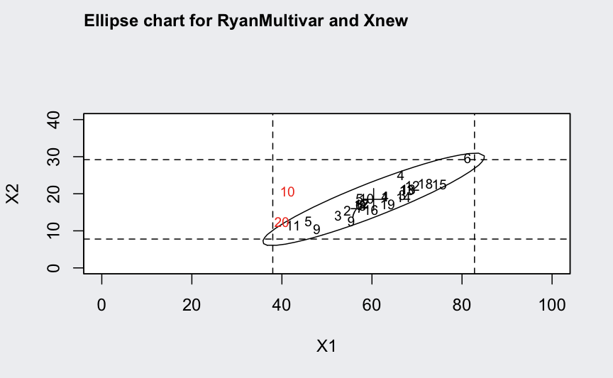
Generate new “out of control” data:
Xnew <- list(X1 = matrix(NA, 10, 4), X2 =  matrix(NA, 10, 4))
for(i in 1:4)
   { x <- MASS::mvrnorm(10, mu = 1.2*q$center, Sigma = q$cov)
     Xnew$X1[,i] <- x[,1]
     Xnew$X2[,i] <- x[,2]
   }
(q <- mqcc(RyanMultivar, type = "T2", newdata = Xnew, pred.limits = TRUE))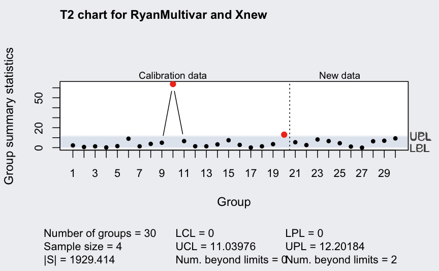
## ── Multivariate Quality Control Chart ────────────
##
## Chart type                 = T2
## Data (phase I)             = RyanMultivar
## Number of groups           = 20
## Group sample size          = 4
## Center =
##      X1      X2
## 60.3750 18.4875
## Covariance matrix =
##          X1        X2
## X1 222.0333 103.11667
## X2 103.1167  56.57917
## |S| = 1929.414
##
## New data (phase II)        = Xnew
## Number of groups           = 10
## Group sample size          = 4
##
## Control limits:
##  LCL      UCL
##    0 11.03976
##
## Prediction limits:
##  LPL      UPL
##    0 12.20184
ellipseChart(q, show.id = TRUE)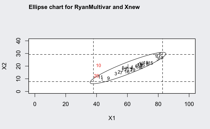
Individual observations data:
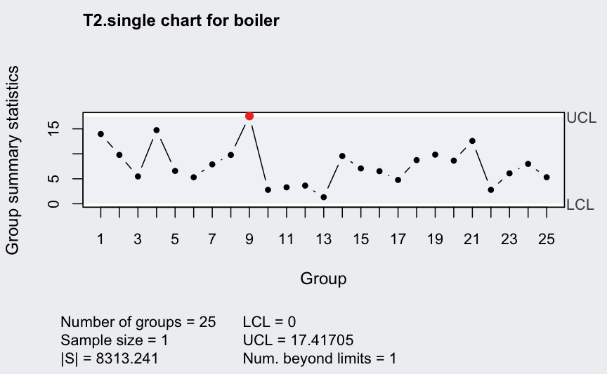
## ── Multivariate Quality Control Chart ────────────
##
## Chart type                 = T2.single
## Data (phase I)             = boiler
## Number of groups           = 25
## Group sample size          = 1
## Center =
##     t1     t2     t3     t4     t5     t6     t7     t8
## 525.00 513.56 538.92 521.68 503.80 512.44 478.72 477.24
## Covariance matrix =
##            t1        t2        t3         t4         t5         t6         t7
## t1 54.0000000 0.9583333 20.583333 31.2916667 20.3333333 -2.2916667 20.3750000
## t2  0.9583333 4.8400000  2.963333  2.6866667  0.3250000  3.0766667  0.7050000
## t3 20.5833333 2.9633333 22.993333 10.0566667  4.9833333  2.0366667  6.4766667
## t4 31.2916667 2.6866667 10.056667 22.3100000 13.5583333 -2.2700000 12.6983333
## t5 20.3333333 0.3250000  4.983333 13.5583333 11.4166667 -1.6583333 10.6500000
## t6 -2.2916667 3.0766667  2.036667 -2.2700000 -1.6583333  4.5066667 -0.7466667
## t7 20.3750000 0.7050000  6.476667 12.6983333 10.6500000 -0.7466667 11.6266667
## t8  0.2083333 3.4433333  2.770000  0.1633333 -0.2833333  3.7233333  0.5283333
##            t8
## t1  0.2083333
## t2  3.4433333
## t3  2.7700000
## t4  0.1633333
## t5 -0.2833333
## t6  3.7233333
## t7  0.5283333
## t8  3.8566667
## |S| = 8313.241
##
## Control limits:
##  LCL      UCL
##    0 17.41705
Generate new “in control” data:
boilerNew <- MASS::mvrnorm(10, mu = q$center, Sigma = q$cov)
mqcc(boiler, type = "T2.single", confidence.level = 0.999,
     newdata = boilerNew, pred.limits = TRUE)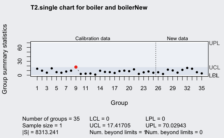
## ── Multivariate Quality Control Chart ────────────
##
## Chart type                 = T2.single
## Data (phase I)             = boiler
## Number of groups           = 25
## Group sample size          = 1
## Center =
##     t1     t2     t3     t4     t5     t6     t7     t8
## 525.00 513.56 538.92 521.68 503.80 512.44 478.72 477.24
## Covariance matrix =
##            t1        t2        t3         t4         t5         t6         t7
## t1 54.0000000 0.9583333 20.583333 31.2916667 20.3333333 -2.2916667 20.3750000
## t2  0.9583333 4.8400000  2.963333  2.6866667  0.3250000  3.0766667  0.7050000
## t3 20.5833333 2.9633333 22.993333 10.0566667  4.9833333  2.0366667  6.4766667
## t4 31.2916667 2.6866667 10.056667 22.3100000 13.5583333 -2.2700000 12.6983333
## t5 20.3333333 0.3250000  4.983333 13.5583333 11.4166667 -1.6583333 10.6500000
## t6 -2.2916667 3.0766667  2.036667 -2.2700000 -1.6583333  4.5066667 -0.7466667
## t7 20.3750000 0.7050000  6.476667 12.6983333 10.6500000 -0.7466667 11.6266667
## t8  0.2083333 3.4433333  2.770000  0.1633333 -0.2833333  3.7233333  0.5283333
##            t8
## t1  0.2083333
## t2  3.4433333
## t3  2.7700000
## t4  0.1633333
## t5 -0.2833333
## t6  3.7233333
## t7  0.5283333
## t8  3.8566667
## |S| = 8313.241
##
## New data (phase II)        = boilerNew
## Number of groups           = 10
## Group sample size          = 1
##
## Control limits:
##  LCL      UCL
##    0 17.41705
##
## Prediction limits:
##  LPL      UPL
##    0 70.02943
Generate new “out of control” data:
boilerNew <- MASS::mvrnorm(10, mu = 1.01*q$center, Sigma = q$cov)
mqcc(boiler, type = "T2.single", confidence.level = 0.999,
     newdata = boilerNew, pred.limits = TRUE)
## ── Multivariate Quality Control Chart ────────────
##
## Chart type                 = T2.single
## Data (phase I)             = boiler
## Number of groups           = 25
## Group sample size          = 1
## Center =
##     t1     t2     t3     t4     t5     t6     t7     t8
## 525.00 513.56 538.92 521.68 503.80 512.44 478.72 477.24
## Covariance matrix =
##            t1        t2        t3         t4         t5         t6         t7
## t1 54.0000000 0.9583333 20.583333 31.2916667 20.3333333 -2.2916667 20.3750000
## t2  0.9583333 4.8400000  2.963333  2.6866667  0.3250000  3.0766667  0.7050000
## t3 20.5833333 2.9633333 22.993333 10.0566667  4.9833333  2.0366667  6.4766667
## t4 31.2916667 2.6866667 10.056667 22.3100000 13.5583333 -2.2700000 12.6983333
## t5 20.3333333 0.3250000  4.983333 13.5583333 11.4166667 -1.6583333 10.6500000
## t6 -2.2916667 3.0766667  2.036667 -2.2700000 -1.6583333  4.5066667 -0.7466667
## t7 20.3750000 0.7050000  6.476667 12.6983333 10.6500000 -0.7466667 11.6266667
## t8  0.2083333 3.4433333  2.770000  0.1633333 -0.2833333  3.7233333  0.5283333
##            t8
## t1  0.2083333
## t2  3.4433333
## t3  2.7700000
## t4  0.1633333
## t5 -0.2833333
## t6  3.7233333
## t7  0.5283333
## t8  3.8566667
## |S| = 8313.241
##
## New data (phase II)        = boilerNew
## Number of groups           = 10
## Group sample size          = 1
##
## Control limits:
##  LCL      UCL
##    0 17.41705
##
## Prediction limits:
##  LPL      UPL
##    0 70.02943
Recompute by providing “robust” estimates for the means and the covariance matrix:
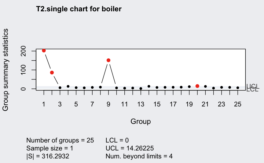
## ── Multivariate Quality Control Chart ────────────
##
## Chart type                 = T2.single
## Data (phase I)             = boiler
## Number of groups           = 25
## Group sample size          = 1
## Center =
##       t1       t2       t3       t4       t5       t6       t7       t8
## 526.0455 513.4545 540.2273 521.7727 503.9091 512.5909 479.0000 477.3636
## Covariance matrix =
##           t1        t2         t3         t4         t5         t6         t7
## t1 34.045455 2.7878788 12.3701299 25.7251082 16.2900433 -4.5043290 14.2857143
## t2  2.787879 5.2121212  4.9870130  3.4891775  0.8051948  3.5281385  1.4761905
## t3 12.370130 4.9870130 10.3744589 10.9112554  4.4978355  0.9545455  4.1428571
## t4 25.725108 3.4891775 10.9112554 20.7554113 12.4069264 -3.0021645 11.0476190
## t5 16.290043 0.8051948  4.4978355 12.4069264 10.9437229 -2.1341991  9.7142857
## t6 -4.504329 3.5281385  0.9545455 -3.0021645 -2.1341991  4.8246753 -1.2857143
## t7 14.285714 1.4761905  4.1428571 11.0476190  9.7142857 -1.2857143 10.1904762
## t8 -1.398268 3.9220779  2.1038961 -0.1991342 -0.5367965  3.9653680  0.2380952
##            t8
## t1 -1.3982684
## t2  3.9220779
## t3  2.1038961
## t4 -0.1991342
## t5 -0.5367965
## t6  3.9653680
## t7  0.2380952
## t8  4.1471861
## |S| = 316.2932
##
## Control limits:
##  LCL      UCL
##    0 14.26225
Pareto chart
defect <- c(80, 27, 66, 94, 33)
names(defect) <- c("price code", "schedule date", "supplier code", "contact num.", "part num.")
(pc = paretoChart(defect, ylab = "Error frequency"))
## ── Pareto Chart ──────────────────────────────────
##
## defect          Frequency Cum.Freq. Percentage Cum.Percent.
##   contact num.         94        94      31.33        31.33
##   price code           80       174      26.67        58.00
##   supplier code        66       240      22.00        80.00
##   part num.            33       273      11.00        91.00
##   schedule date        27       300       9.00       100.00
plot(pc)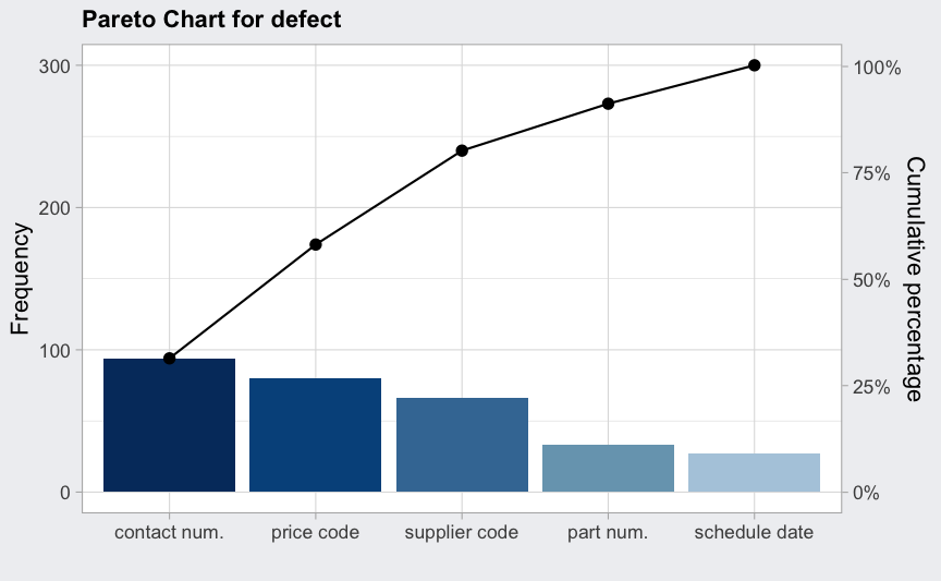
Cause and effect diagram
causeEffectDiagram(cause = list(Measurements = c("Micrometers",
                                                 "Microscopes",
                                                 "Inspectors"),
                                Materials = c("Alloys",
                                              "Lubricants",
                                              "Suppliers"),
                                Personnel = c("Shifts",
                                              "Supervisors",
                                              "Training",
                                              "Operators"),
                                Environment = c("Condensation",
                                                "Moisture"),
                                Methods = c("Brake",
                                            "Engager",
                                            "Angle"),
                                Machines = c("Speed",
                                             "Lathes",
                                             "Bits",
                                             "Sockets")),
                   effect = "Surface Flaws")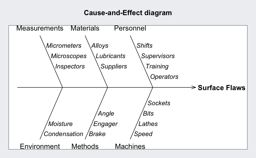
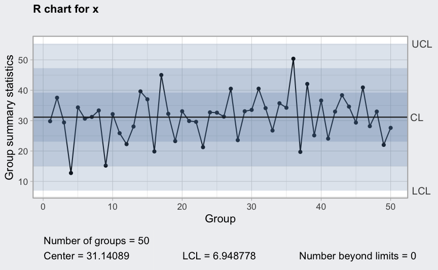
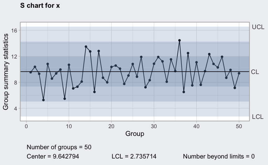
Process variation examples
In the following simulated data are used to describe some models for process variation. For further details see Wetherill, G.B. and Brown, D.W. (1991) Statistical Process Control, New York, Chapman and Hall, Chapter 3.
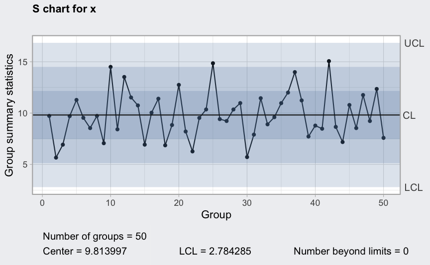
Simple random variation
mu <- 100
sigma_W <- 10
epsilon <- rnorm(500)
x <- matrix(mu + sigma_W*epsilon, ncol = 10, byrow = TRUE)
plot(qcc(x, type = "xbar", rules = 1:4))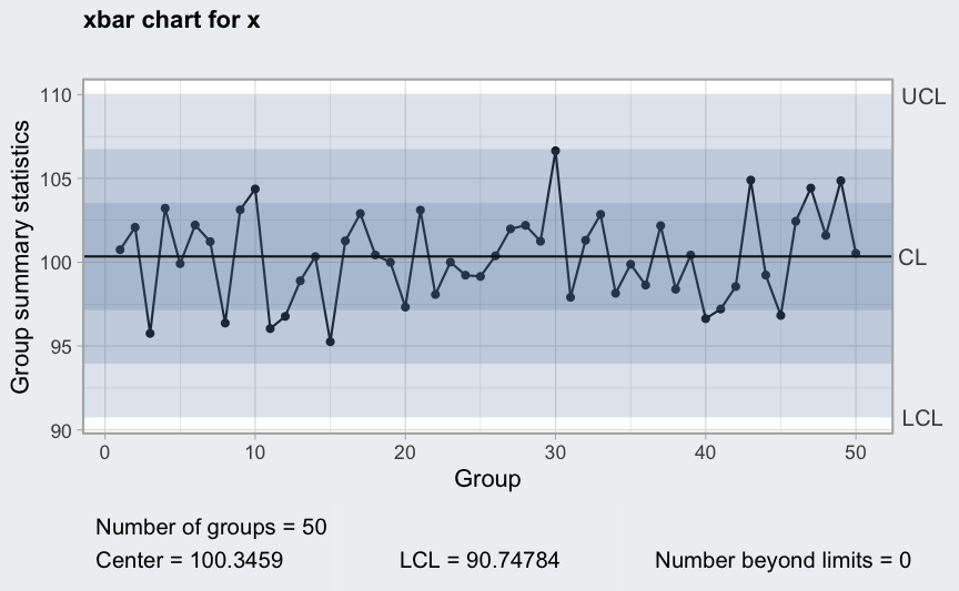
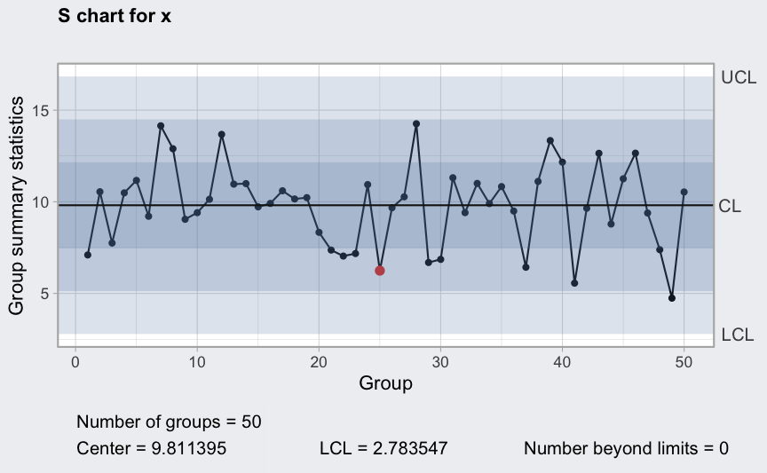
Between and within sample extra variation
mu <- 100
sigma_W <- 10
sigma_B <- 5
epsilon <- rnorm(500)
u <- as.vector(sapply(rnorm(50), rep, 10))
x <- mu + sigma_B*u + sigma_W*epsilon
x <- matrix(x, ncol = 10, byrow = TRUE)
plot(qcc(x, type = "xbar", rules = 1:4))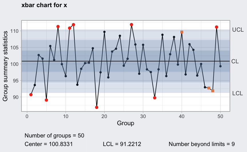
Autocorrelation
where
,
and
.
mu <- 100
rho <- 0.9
sigma_W <- 10
sigma_B <- 5
epsilon <- rnorm(500)
u <- rnorm(500)
W <- rep(0,100)
for(i in 2:length(W))
  W[i] <- rho*W[i-1] + sigma_B*u[i]
x <- mu + sigma_B*u + sigma_W*epsilon
x <- matrix(x, ncol = 10, byrow = TRUE)
plot(qcc(x, type = "xbar", rules = 1:4))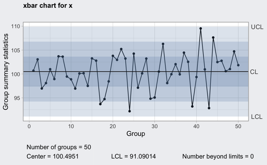

Recurring cycles
Assume we have 3 working turns of 8 hours each for each working day, so points in time, and at each point we sample 5 units.
where
()
is the cycle.
mu <- 100
sigma_W <- 10
epsilon <- rnorm(120, sd = 0.3)
W <- c(-4, 0, 1, 2, 4, 2, 0, -2) # assumed workers cycle
W <- rep(rep(W, rep(5,8)), 3)
x <- mu + W + sigma_W*epsilon
x <- matrix(x, ncol = 5, byrow = TRUE)
plot(qcc(x, type = "xbar", rules = 1:4))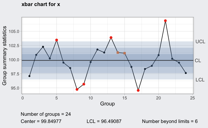

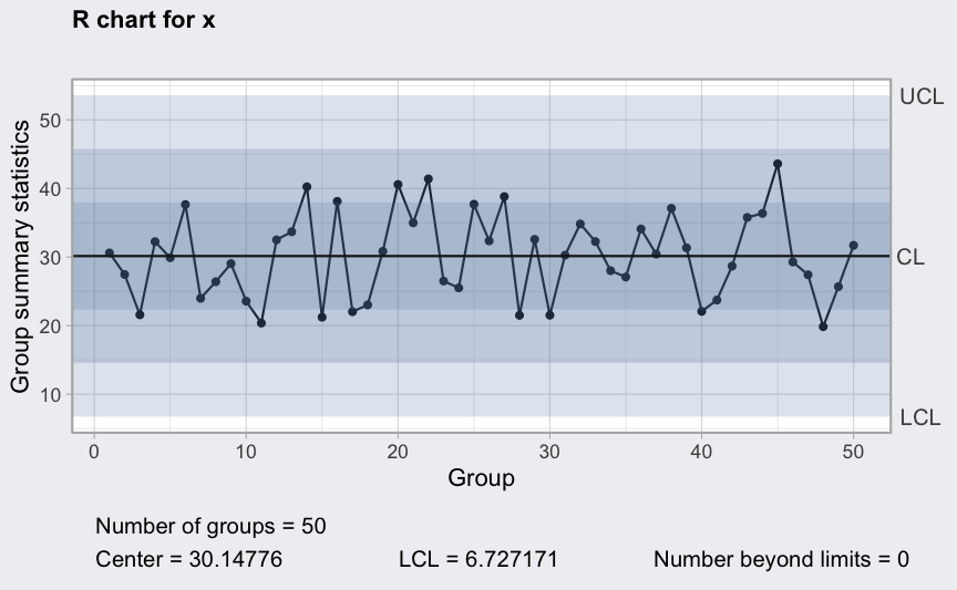
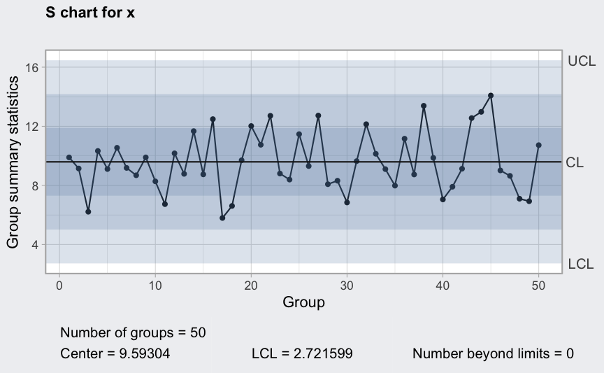
Trends
where
mu <- 100
sigma_W <- 10
epsilon <- rnorm(500)
W <- rep(0.2*1:100, rep(5,100))
x <- mu + W + sigma_W*epsilon
x <- matrix(x, ncol = 10, byrow = TRUE)
plot(qcc(x, type = "xbar", rules = 1:4))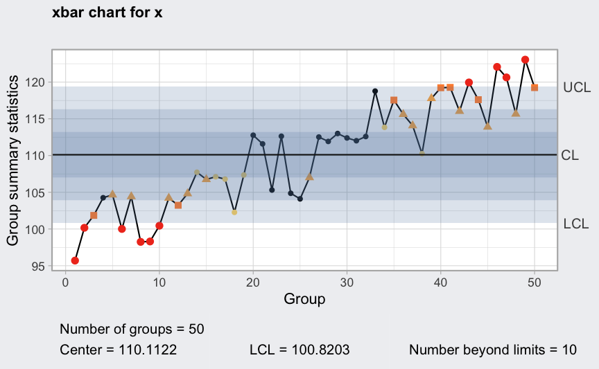
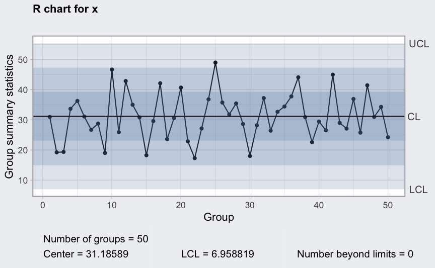
Mixture
where
.
mu1 <- 90
mu2 <- 110
sigma_W <- 10
epsilon <- rnorm(500)
p <- rbinom(50, 1, 0.5)
mu <- mu1*p + mu2*(1-p)
x <- rep(mu, rep(10, length(mu))) + sigma_W*epsilon
x <- matrix(x, ncol = 10, byrow = TRUE)
plot(qcc(x, type = "xbar", rules = 1:4))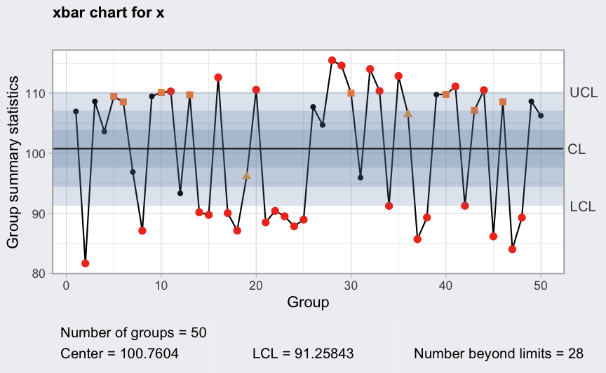
References
Montgomery, D.C. (2013) Introduction to Statistical Quality Control, 7th ed. New York: John Wiley & Sons.
Ryan, T. P. (2011), Statistical Methods for Quality Improvement, 3rd ed. New York: John Wiley & Sons.
Scrucca, L. (2004) qcc: an R package for quality control charting and statistical process control. R News 4/1, 11-17.
sessionInfo()
## R version 4.5.2 (2025-10-31)
## Platform: aarch64-apple-darwin20
## Running under: macOS Sequoia 15.6.1
##
## Matrix products: default
## BLAS:   /System/Library/Frameworks/Accelerate.framework/Versions/A/Frameworks/vecLib.framework/Versions/A/libBLAS.dylib
## LAPACK: /Library/Frameworks/R.framework/Versions/4.5-arm64/Resources/lib/libRlapack.dylib;  LAPACK version 3.12.1
##
## locale:
## [1] en_US.UTF-8/en_US.UTF-8/en_US.UTF-8/C/en_US.UTF-8/en_US.UTF-8
##
## time zone: Europe/Rome
## tzcode source: internal
##
## attached base packages:
## [1] stats     graphics  grDevices utils     datasets  methods   base
##
## other attached packages:
## [1] qcc_3.0         patchwork_1.3.2 ggplot2_4.0.0   knitr_1.50
##
## loaded via a namespace (and not attached):
##  [1] crayon_1.5.3       vctrs_0.6.5        cli_3.6.5          rlang_1.1.6
##  [5] xfun_0.53          generics_0.1.4     S7_0.2.0           jsonlite_2.0.0
##  [9] labeling_0.4.3     glue_1.8.0         htmltools_0.5.8.1  sass_0.4.10
## [13] scales_1.4.0       rmarkdown_2.30     grid_4.5.2         tibble_3.3.0
## [17] evaluate_1.0.5     jquerylib_0.1.4    MASS_7.3-65        fastmap_1.2.0
## [21] yaml_2.3.10        lifecycle_1.0.4    compiler_4.5.2     dplyr_1.1.4
## [25] fs_1.6.6           RColorBrewer_1.1-3 pkgconfig_2.0.3    htmlwidgets_1.6.4
## [29] rstudioapi_0.17.1  farver_2.1.2       digest_0.6.37      R6_2.6.1
## [33] tidyselect_1.2.1   pillar_1.11.1      magrittr_2.0.4     bslib_0.9.0
## [37] withr_3.0.2        tools_4.5.2        gtable_0.3.6       pkgdown_2.1.3
## [41] cachem_1.1.0       desc_1.4.3